UML-08: Anomaly Detection

Publish on: 2022/10/08 Classify at: CODE/Unsupervised Machine Learning

Words: 1629 Read:≈ 8min

Summary

Master Anomaly Detection: The 'Rare Species Hunter'. Learn how Isolation Forest (20 Questions) and LOF (Loneliness Index) find outliers in your data.

Learning Objectives

After reading this post, you will be able to:

Understand the three main approaches to anomaly detection
Implement Isolation Forest and Local Outlier Factor
Know when to use each anomaly detection method
Handle contamination rate and threshold selection

Theory

The Intuition: The Rare Species Hunter

Imagine you are a biologist exploring a new island.

Normal Data (Sparrows): You see thousands of small, brown birds. They are everywhere and look mostly the same.
Anomalies (The Phoenix): Suddenly, you see a giant, glowing red bird. It stands out immediately.

Anomaly Detection is the set of algorithms designed to find these “Rare Species” in a sea of common data, without knowing beforehand what they look like.

graph LR A["📊 Data"] --> B["🔍 Anomaly Detector"] B --> C["✅ Normal"] B --> D["⚠️ Anomaly"] style C fill:#c8e6c9 style D fill:#ffcdd2

Applications:

🏦 Fraud detection (unusual transactions)
🖥️ System monitoring (server failures)
🏭 Quality control (defective products)
🏥 Medical diagnosis (rare diseases)

Three Approaches to Anomaly Detection

Approach	Method	Assumption
Statistical	Z-score, IQR	Data follows known distribution
Distance-based	LOF, k-NN	Anomalies are far from neighbors
Tree-based	Isolation Forest	Anomalies are easier to isolate

Statistical Methods

Z-Score

Points with $|z| > 3$ are often considered anomalies:

$$z = \frac{x - \mu}{\sigma}$$

Interquartile Range (IQR)

Points outside the “fences” are outliers:

Lower fence: $Q_1 - 1.5 \times IQR$
Upper fence: $Q_3 + 1.5 \times IQR$

The “Square Peg” Problem (Why Z-Score Fails)

Z-score looks at features individually.

Imagine a person who is 6'0" (Normal).
Imagine a person who weighs 100 lbs (Normal).
But a person who is 6'0" AND 100 lbs? That’s an anomaly! Z-score might miss this because each dimension alone looks fine. It can’t see the relationship between features.

Isolation Forest: The “20 Questions” Game

Think of this as playing “20 Questions” to identify an animal.

To identify a Sparrow (Standard Point): You need many questions. “Is it small? Yes. Brown? Yes. Beak shape? Conical…” because so many birds fit this description.
To identify a Phoenix (Anomaly): You need only one question. “Is it on fire? Yes.” -> Found it!

Isolation Forest builds random decision trees.

Anomalies are distinct, so they get “isolated” near the root of the tree (few splits).
Normal points are clustered together, so they end up deep in the leaves (many splits).

graph LR subgraph cluster_tree ["Random Decision Tree"] direction LR A["Root: Is it on fire?"] B["🔥 Yes (Anomaly)"] C["No (Normal Cluster)"] D["Is it small?"] E["Is it brown?"] F["🐦 Sparrow"] end A -->|Short Path| B A --> C --> D --> E --> F style B fill:#ffcdd2 style F fill:#c8e6c9

Why it works: The “Outsider” Principle

Because anomalies are " different" and “few”, random cuts are very likely to separate them from the rest of the data early on.

Normal points are crowded together. You have to peel away many layers (cuts) to isolate one specific normal point.
Anomalies sit alone. One or two random cuts are usually enough to fence them off.

Algorithm:

Build many random trees (random splits on random features)
Anomalies require fewer splits to be isolated
Score = average path length across all trees

Anomaly Score: $$s(x, n) = 2^{-\frac{E[h(x)]}{c(n)}}$$

where $h(x)$ = path length, $c(n)$ = average path length in random trees.

Score ≈ 1: anomaly
Score ≈ 0: normal
Score ≈ 0.5: uncertain

Isolation Forest concept — Anomalies (red) require fewer splits to isolate than normal points (blue)

Local Outlier Factor (LOF): The “Loneliness” Index

LOF measures how isolated a point is compared to its neighbors.

The Crowd (High Density): A penguin in a flock is happy because its neighbors are just as close to each other as they are to him.
The Loner (Low Density): A penguin alone on an iceberg is lonely. His density is low, while his nearest neighbors (far away in the flock) have high density.

LOF » 1 means the point is in a lower-density region than its neighbors (Anomaly).

$$LOF(x) = \frac{\text{avg neighbor density}}{\text{density at } x}$$

LOF ≈ 1: similar density to neighbors (normal)
LOF » 1: lower density than neighbors (anomaly)

LOF concept — LOF detects local outliers by comparing density to neighbors

Why LOF? The “Density Problem” Imagine two clusters:

City (High Density): Points are packed tight. An anomaly here might be just a block away.
Countryside (Low Density): Points represent farms miles apart.

A global method (like k-NN distance) might flag all the farms as anomalies because they are far apart. LOF adapts: It knows that being 1 mile apart is “normal” in the countryside, but “anomalous” in the city.

Code Practice

Statistical Anomaly Detection

🐍 Python

 1
 2
 3
 4
 5
 6
 7
 8
 9
10
11
12
13
14
15
16
17
18
19
20
21
22
23
24
25
import numpy as np
import matplotlib.pyplot as plt
from scipy import stats

# Generate data with outliers
np.random.seed(42)
normal_data = np.random.normal(0, 1, 1000)
outliers = np.array([-5, -4.5, 4.5, 5, 5.5])
data = np.concatenate([normal_data, outliers])

# Z-score method
z_scores = np.abs(stats.zscore(data))
z_outliers = z_scores > 3

# IQR method
Q1, Q3 = np.percentile(data, [25, 75])
IQR = Q3 - Q1
iqr_outliers = (data < Q1 - 1.5*IQR) | (data > Q3 + 1.5*IQR)

print("=" * 50)
print("STATISTICAL ANOMALY DETECTION")
print("=" * 50)
print(f"\n📊 Total points: {len(data)}")
print(f"📍 Z-score outliers: {z_outliers.sum()}")
print(f"📍 IQR outliers: {iqr_outliers.sum()}")

Output:

1
2
3
4
5
6
7
==================================================
STATISTICAL ANOMALY DETECTION
==================================================

📊 Total points: 1005
📍 Z-score outliers: 7
📍 IQR outliers: 13

Isolation Forest

🐍 Python

 1
 2
 3
 4
 5
 6
 7
 8
 9
10
11
12
13
14
15
16
17
18
19
20
21
from sklearn.ensemble import IsolationForest
from sklearn.datasets import make_blobs

# Generate 2D data with anomalies
np.random.seed(42)
X_normal, _ = make_blobs(n_samples=300, centers=1, cluster_std=0.5, random_state=42)
X_outliers = np.random.uniform(-4, 4, (20, 2))
X = np.vstack([X_normal, X_outliers])

# Fit Isolation Forest
# contamination=0.06: We expect ~6% of rare beasts in the flock
iso_forest = IsolationForest(contamination=0.06, random_state=42)
predictions = iso_forest.fit_predict(X)
scores = iso_forest.decision_function(X)

print("=" * 50)
print("ISOLATION FOREST")
print("=" * 50)
print(f"\n📊 Total points: {len(X)}")
print(f"⚠️ Detected anomalies: {(predictions == -1).sum()}")
print(f"📈 Score range: [{scores.min():.3f}, {scores.max():.3f}]")

Output:

1
2
3
4
5
6
7
==================================================
ISOLATION FOREST
==================================================

📊 Total points: 320
⚠️ Detected anomalies: 20
📈 Score range: [-0.145, 0.290]

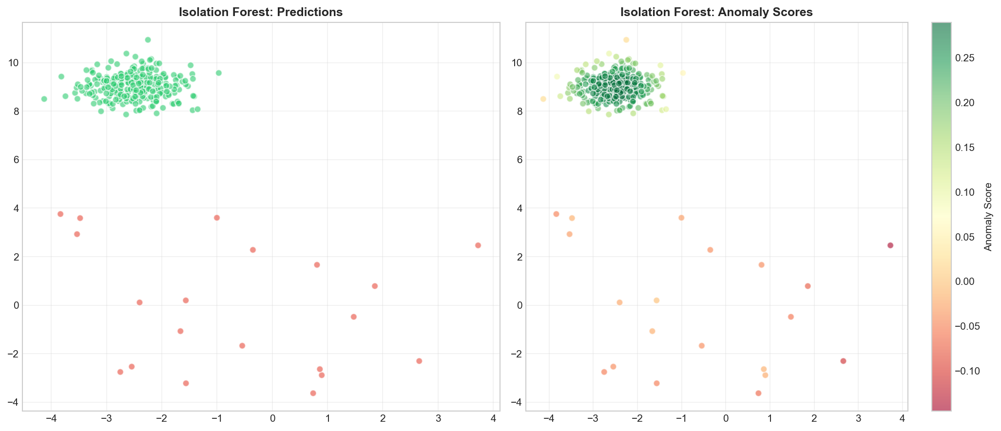
Visualizing Isolation Forest

🐍 Python

 1
 2
 3
 4
 5
 6
 7
 8
 9
10
11
12
13
14
15
16
17
18
19
fig, axes = plt.subplots(1, 2, figsize=(14, 6))

# Predictions
colors = ['#2ecc71' if p == 1 else '#e74c3c' for p in predictions]
axes[0].scatter(X[:, 0], X[:, 1], c=colors, alpha=0.6, s=40, edgecolors='white')
axes[0].set_title('Isolation Forest: Predictions', fontsize=12, fontweight='bold')
axes[0].legend(['Normal', 'Anomaly'], loc='upper right')
axes[0].grid(True, alpha=0.3)

# Anomaly scores
scatter = axes[1].scatter(X[:, 0], X[:, 1], c=scores, cmap='RdYlGn', 
                          alpha=0.6, s=40, edgecolors='white')
plt.colorbar(scatter, ax=axes[1], label='Anomaly Score')
axes[1].set_title('Isolation Forest: Anomaly Scores', fontsize=12, fontweight='bold')
axes[1].grid(True, alpha=0.3)

plt.tight_layout()
plt.savefig('assets/isolation_forest.png', dpi=150)
plt.show()

Isolation Forest results — Left: detected anomalies (red). Right: anomaly scores (red = high, green = low)

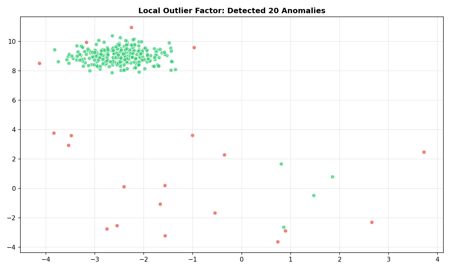
Local Outlier Factor

🐍 Python

 1
 2
 3
 4
 5
 6
 7
 8
 9
10
11
12
13
14
15
16
17
18
19
20
21
22
from sklearn.neighbors import LocalOutlierFactor

# Fit LOF
lof = LocalOutlierFactor(n_neighbors=20, contamination=0.06)
predictions_lof = lof.fit_predict(X)
lof_scores = lof.negative_outlier_factor_

print("=" * 50)
print("LOCAL OUTLIER FACTOR")
print("=" * 50)
print(f"\n📊 Total points: {len(X)}")
print(f"⚠️ Detected anomalies: {(predictions_lof == -1).sum()}")
print(f"📈 LOF scores range: [{lof_scores.min():.3f}, {lof_scores.max():.3f}]")

# Visualize Results
plt.figure(figsize=(10, 6))
colors = ['#2ecc71' if p == 1 else '#e74c3c' for p in predictions_lof]
plt.scatter(X[:, 0], X[:, 1], c=colors, alpha=0.7, s=40, edgecolors='white')
plt.title(f'Local Outlier Factor: Detected {(predictions_lof == -1).sum()} Anomalies', fontsize=12, fontweight='bold')
plt.grid(True, alpha=0.3)
plt.savefig('assets/lof_concept.png', dpi=150)
plt.show()

Output:

1
2
3
4
5
6
7
==================================================
LOCAL OUTLIER FACTOR
==================================================

📊 Total points: 320
⚠️ Detected anomalies: 20
📈 LOF scores range: [-8.501, -0.959]

LOF results — LOF detects anomalies based on local density comparison

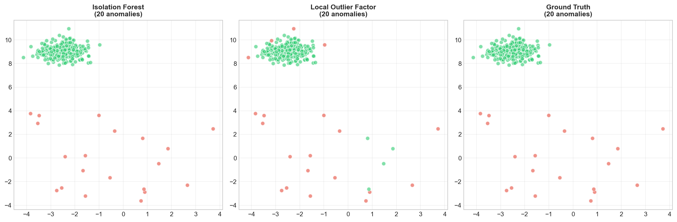
Comparing Methods

🐍 Python

 1
 2
 3
 4
 5
 6
 7
 8
 9
10
11
12
13
14
15
16
17
18
19
20
21
22
23
24
fig, axes = plt.subplots(1, 3, figsize=(15, 5))

# Isolation Forest
axes[0].scatter(X[:, 0], X[:, 1], c=['#2ecc71' if p == 1 else '#e74c3c' for p in predictions],
                alpha=0.6, s=40, edgecolors='white')
axes[0].set_title(f'Isolation Forest\n({(predictions == -1).sum()} anomalies)', fontsize=11, fontweight='bold')
axes[0].grid(True, alpha=0.3)

# LOF
axes[1].scatter(X[:, 0], X[:, 1], c=['#2ecc71' if p == 1 else '#e74c3c' for p in predictions_lof],
                alpha=0.6, s=40, edgecolors='white')
axes[1].set_title(f'Local Outlier Factor\n({(predictions_lof == -1).sum()} anomalies)', fontsize=11, fontweight='bold')
axes[1].grid(True, alpha=0.3)

# Ground truth
true_labels = np.concatenate([np.ones(300), -np.ones(20)])
axes[2].scatter(X[:, 0], X[:, 1], c=['#2ecc71' if p == 1 else '#e74c3c' for p in true_labels],
                alpha=0.6, s=40, edgecolors='white')
axes[2].set_title('Ground Truth\n(20 anomalies)', fontsize=11, fontweight='bold')
axes[2].grid(True, alpha=0.3)

plt.tight_layout()
plt.savefig('assets/method_comparison.png', dpi=150)
plt.show()

Comparison of anomaly methods — Both methods correctly identify most outliers

Deep Dive

Choosing the Right Method

Method	Best For	Limitations
Z-score/IQR	Univariate, Gaussian data	Assumes distribution
Isolation Forest	High-dimensional, fast	Global outliers
LOF	Local outliers, varied densities	Slower, needs k choice
One-Class SVM	Complex boundaries	Scaling, parameters

Handling Contamination Rate

The contamination parameter is crucial but often unknown:

If known: set explicitly (e.g., 5% fraud rate)
If unknown: try multiple values, use domain knowledge
Alternative: use auto and threshold scores manually

Frequently Asked Questions

Q1: How do I evaluate anomaly detection without labels?

Difficult! Options:

Manual inspection of flagged anomalies
Domain expert validation
If partial labels exist: precision/recall on known anomalies

Q2: What if I have labeled anomalies?

Then you have a supervised classification problem! Consider:

One-Class SVM (trained on normals only)
Supervised classifiers with class imbalance handling

Q3: How do I handle high-dimensional data?

Use Isolation Forest (handles high-D well)
Apply PCA first, then anomaly detection
Use distance metrics designed for high-D (e.g., cosine)

Summary

Concept	Key Points
Anomaly	Unusual observation, differs from majority
Isolation Forest	Tree-based, isolates anomalies quickly
LOF	Density-based, compares to local neighborhood
Contamination	Expected proportion of anomalies
Evaluation	Difficult without labels; use domain knowledge

References

Liu, F.T. et al. (2008). “Isolation Forest”
Breunig, M.M. et al. (2000). “LOF: Identifying Density-Based Local Outliers”
sklearn Outlier Detection