Learning Objectives

After reading this post, you will be able to:

• Understand t-SNE’s approach to preserving local structure
• Use UMAP for faster, more scalable visualizations
• Know the key parameters (perplexity, n_neighbors) and their effects
• Choose between PCA, t-SNE, and UMAP for your visualization needs

Theory

The Intuition: The Origami Master

Imagine your data is a piece of paper with a map drawn on it.

• The Manifold: Now crumple that paper into a tight ball. This is your High-Dimensional data. The points that were originally far apart might now be touching in 3D space.
• PCA (The Hammer): PCA tries to simplify this 3D ball by smashing it flat with a hammer. It destroys the original map structure.
• t-SNE / UMAP (The Unfolder): These algorithms are like Origami Masters. They carefully unfold the crumpled ball, smoothing it out to reveal the original 2D map.

Manifold Learning is the art of unfolding this structure.

The Problem: Distance is a Lie

In the crumpled paper ball, point A (top of a fold) might physically touch point B (bottom of a fold).

• Euclidean Distance (Straight line): Says they are neighbors (Distance = 0).
• Geodesic Distance (Along the paper): Walking along the surface, they are actually very far apart!

Key Insight: PCA uses the straight-line distance, which is why it gets confused by the fold. t-SNE and UMAP try to respect the “walking distance” along the paper surface.

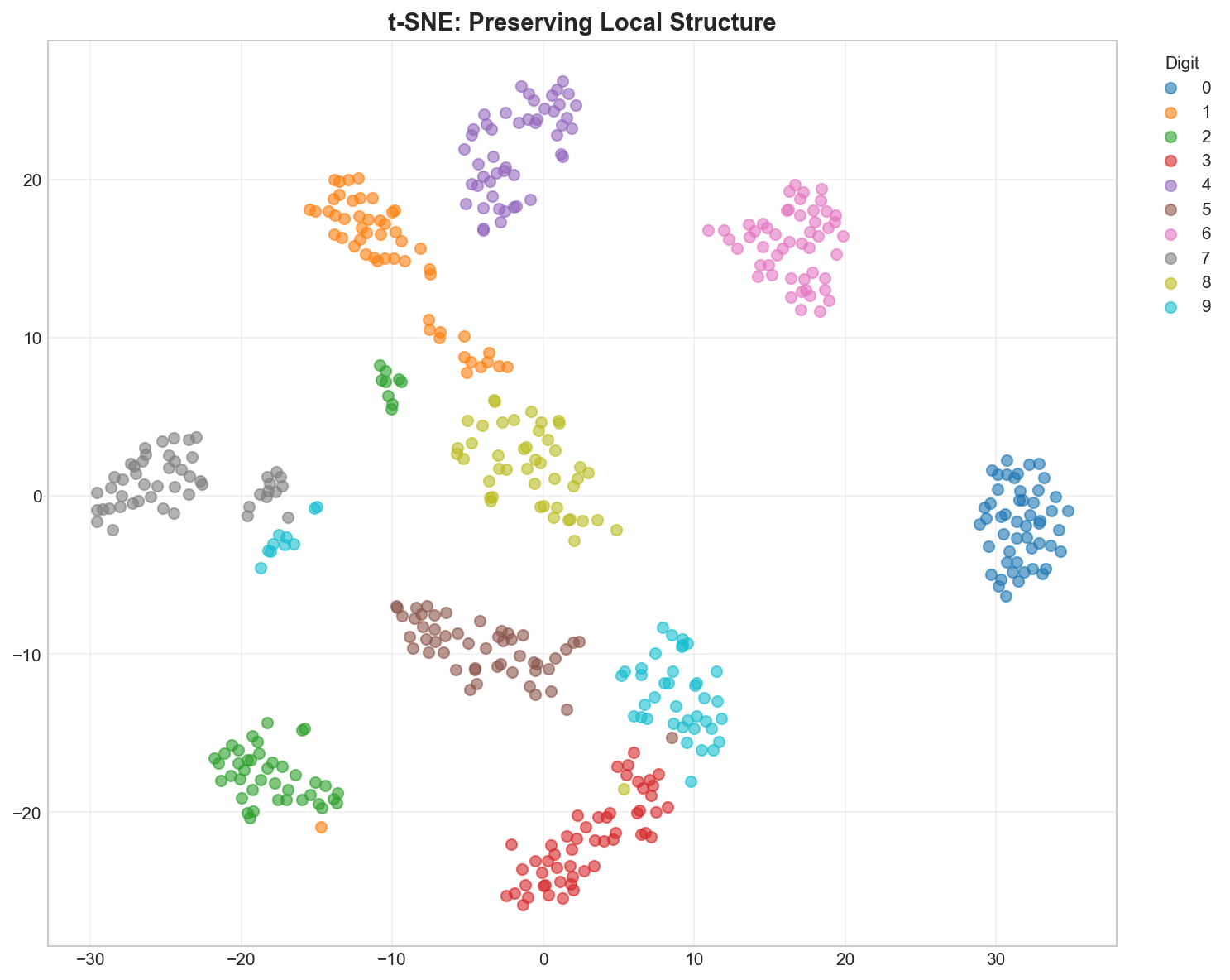
t-SNE: The Social Event Planner

Think of t-SNE as trying to recreate a cocktail party seating plan.

1. High-D Space (The Party): People are mingling freely in a large room.
   • Everyone picks their “Best Friends” (Perplexity = 30 neighbors).
   • You are very close to your clique.
2. Low-D Space (The Seating Chart): You have to seat everyone at a small 2D table.
   • The Goal: If Alice and Bob were standing together at the party (High probability), they MUST sit together at the table.
   • The Constraint: There isn’t enough room! You have to push non-friends far away to make space for friends to be close.
3. KL Divergence (The Stress): The algorithm measures how “unhappy” everyone is with their seats. It shuffles people around until the “social stress” is minimized.

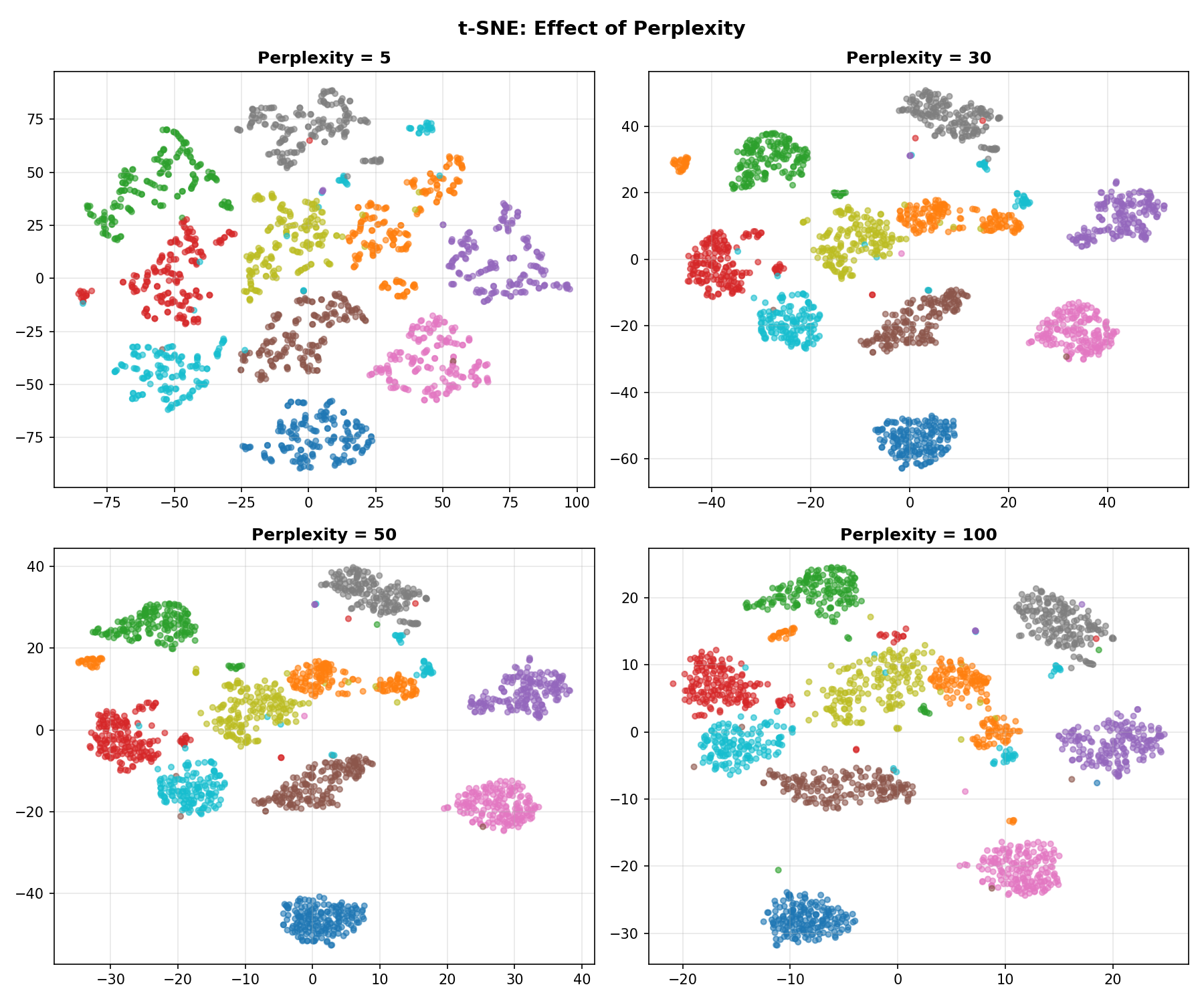
Key Parameter: Perplexity (The Thread Length)

Think of Perplexity as the length of the thread you use to connect points.

• Low (5-10): Short threads. You only connect to your immediate neighbors. The map breaks into many small, unconnected islands.
• High (50+): Long threads. You connect to points far away. Everything gets pulled into one big blob.
• Medium (30): Just right.

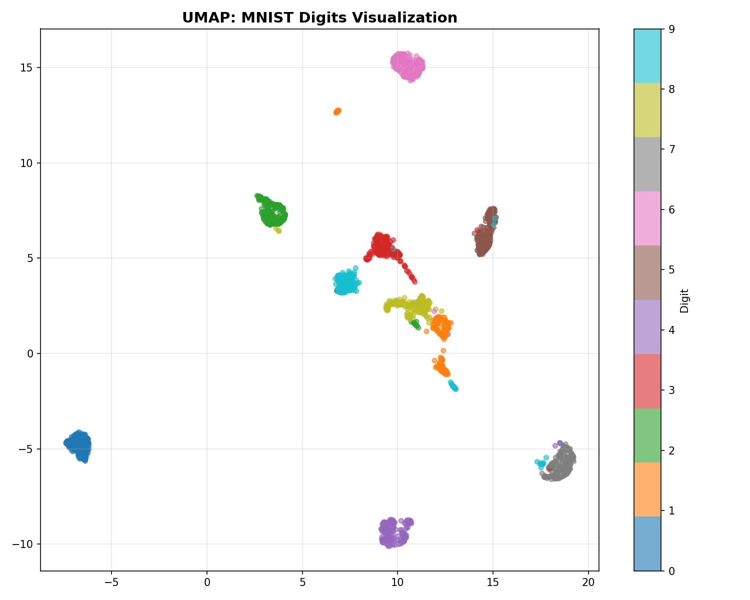
UMAP: The Fast Sketch Artist

UMAP is a newer algorithm. Why is it so popular?

• Speed: t-SNE calculates interactions between every pair of points (slow). UMAP approximates the manifold structure mathematically (topology), avoiding unnecessary calculations. It’s like sketching the shape of the mountain instead of measuring every single rock.
• Global Structure: Because of its mathematical foundation, UMAP is better at keeping far-away clusters in roughly the correct relative positions (e.g., “Continent A is north of Continent B”), whereas t-SNE might put them anywhere.

Code Practice

t-SNE on MNIST Digits

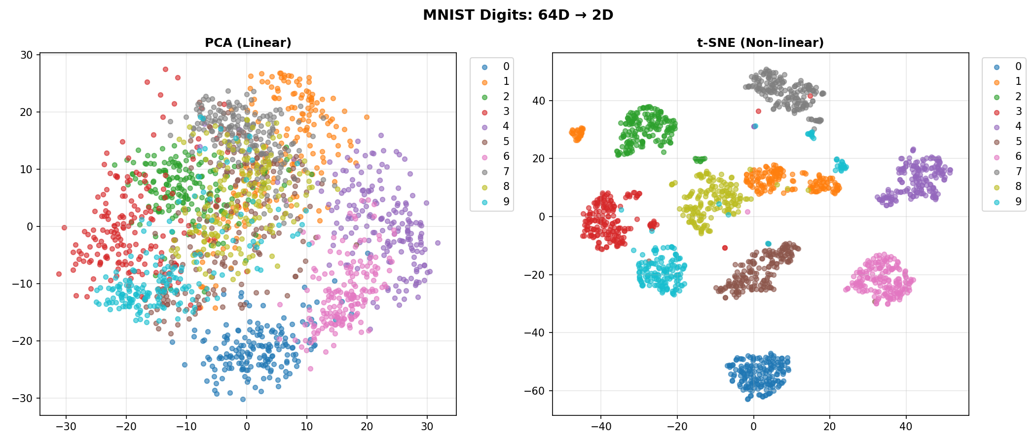
We’ll use the classic MNIST dataset (handwritten digits).

• The Data: 1,797 images of digits (0-9).
• The Dimensions: Each image is 8x8 pixels = 64 dimensions.
• The Goal: Can we unfold this 64-dimensional data into 2 dimensions so that all the “0"s are in one pile and all the “1"s in another?

 1
 2
 3
 4
 5
 6
 7
 8
 9
10
11
12
13
14
15
16
17
18
19
20
21

import numpy as np
import matplotlib.pyplot as plt
from sklearn.datasets import load_digits
from sklearn.manifold import TSNE
from sklearn.decomposition import PCA

# Load data
digits = load_digits()
X, y = digits.data, digits.target

print("=" * 50)
print("t-SNE VISUALIZATION")
print("=" * 50)
print(f"📊 Dataset: {X.shape[0]} samples, {X.shape[1]} dimensions")

# Apply t-SNE
# perplexity=30: Look at ~30 neighbors to decide where to place a point
tsne = TSNE(n_components=2, perplexity=30, random_state=42)
X_tsne = tsne.fit_transform(X)

print(f"📐 Embedded shape: {X_tsne.shape}")

Output:

1
2
3
4
5

==================================================
t-SNE VISUALIZATION
==================================================
📊 Dataset: 1797 samples, 64 dimensions
📐 Embedded shape: (1797, 2)

Comparing PCA vs t-SNE

 1
 2
 3
 4
 5
 6
 7
 8
 9
10
11
12
13
14
15
16
17
18
19
20
21
22
23
24
25
26
27
28
29

# PCA for comparison
pca = PCA(n_components=2)
X_pca = pca.fit_transform(X)

fig, axes = plt.subplots(1, 2, figsize=(14, 6))
colors = plt.cm.tab10(np.linspace(0, 1, 10))

# PCA
for i in range(10):
    mask = y == i
    axes[0].scatter(X_pca[mask, 0], X_pca[mask, 1], c=[colors[i]], 
                    alpha=0.6, s=20, label=str(i))
axes[0].set_title('PCA (Linear)', fontsize=12, fontweight='bold')
axes[0].legend(bbox_to_anchor=(1.02, 1), loc='upper left')
axes[0].grid(True, alpha=0.3)

# t-SNE
for i in range(10):
    mask = y == i
    axes[1].scatter(X_tsne[mask, 0], X_tsne[mask, 1], c=[colors[i]], 
                    alpha=0.6, s=20, label=str(i))
axes[1].set_title('t-SNE (Non-linear)', fontsize=12, fontweight='bold')
axes[1].legend(bbox_to_anchor=(1.02, 1), loc='upper left')
axes[1].grid(True, alpha=0.3)

plt.suptitle('MNIST Digits: 64D → 2D', fontsize=14, fontweight='bold')
plt.tight_layout()
plt.savefig('assets/pca_vs_tsne.png', dpi=150)
plt.show()

UMAP Visualization

 1
 2
 3
 4
 5
 6
 7
 8
 9
10
11
12
13
14
15
16
17

# pip install umap-learn
import umap

# Apply UMAP
reducer = umap.UMAP(n_neighbors=15, min_dist=0.1, random_state=42)
X_umap = reducer.fit_transform(X)

fig, ax = plt.subplots(figsize=(10, 8))
scatter = ax.scatter(X_umap[:, 0], X_umap[:, 1], c=y, cmap='tab10', 
                     alpha=0.6, s=20)
plt.colorbar(scatter, ax=ax, label='Digit')
ax.set_title('UMAP: MNIST Digits Visualization', fontsize=14, fontweight='bold')
ax.grid(True, alpha=0.3)

plt.tight_layout()
plt.savefig('assets/umap_digits.png', dpi=150)
plt.show()

Effect of Perplexity

 1
 2
 3
 4
 5
 6
 7
 8
 9
10
11
12
13
14
15
16
17
18

perplexities = [5, 30, 50, 100]

fig, axes = plt.subplots(2, 2, figsize=(12, 10))
axes = axes.flatten()

for ax, perp in zip(axes, perplexities):
    tsne = TSNE(n_components=2, perplexity=perp, random_state=42)
    X_embedded = tsne.fit_transform(X)
    
    scatter = ax.scatter(X_embedded[:, 0], X_embedded[:, 1], c=y, 
                         cmap='tab10', alpha=0.6, s=15)
    ax.set_title(f'Perplexity = {perp}', fontsize=12, fontweight='bold')
    ax.grid(True, alpha=0.3)

plt.suptitle('t-SNE: Effect of Perplexity', fontsize=14, fontweight='bold')
plt.tight_layout()
plt.savefig('assets/perplexity_effect.png', dpi=150)
plt.show()

Deep Dive

Common Pitfalls

t-SNE / UMAP interpretation warnings:

1. Cluster sizes don’t matter — t-SNE/UMAP distort densities
2. Distances between clusters don’t matter — only local structure is preserved
3. Different runs give different results — always set random_state
4. Don’t use for downstream ML — embeddings are for visualization only

When to Use Each Method

Frequently Asked Questions

Q1: Can I use t-SNE/UMAP embeddings for clustering?

You can, but with caution:

• Cluster on original data, visualize with t-SNE/UMAP
• Or cluster on UMAP (but be aware of distortions)

Q2: My t-SNE looks different every time — why?

t-SNE is stochastic. Always set random_state for reproducibility.

Q3: How do I choose between t-SNE and UMAP?

• t-SNE: Classic choice, widely used in publications
• UMAP: Faster, better global structure, more parameters to tune

Summary

References

• van der Maaten, L. & Hinton, G. (2008). “Visualizing Data using t-SNE”
• McInnes, L. et al. (2018). “UMAP: Uniform Manifold Approximation and Projection”
• sklearn t-SNE
• UMAP Documentation