Learning Objectives

After reading this post, you will be able to:

• Understand PCA as finding directions of maximum variance
• Perform dimensionality reduction for visualization and compression
• Interpret explained variance and choose the number of components
• Know when PCA helps and when it fails

Theory

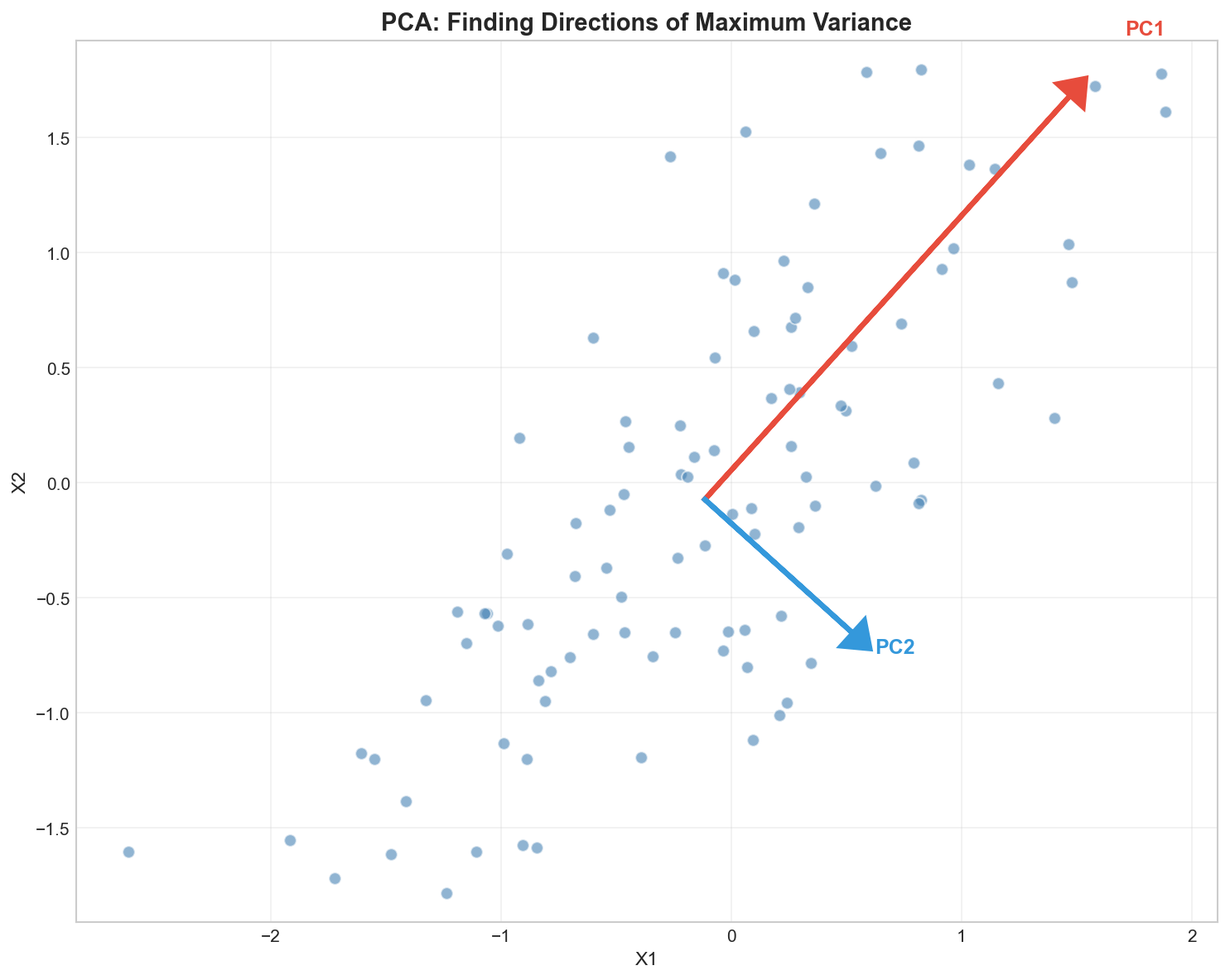
The Intuition: The Photographer’s Challenge

Imagine you are trying to take a photo of a complex 3D object (like a teapot) to put in a catalog. You can only print a flat 2D image, but you want to show as much detail as possible.

• Bad Angle: Taking a photo from directly above might just look like a circle (lid). You lose all the information about the spout and handle.
• Best Angle (PC1): The angle where the teapot looks “widest” and most recognizable. This captures the maximum variance (detail).
• Second Best Angle (PC2): An angle perpendicular to the first one that adds the next most amount of unique detail (e.g., depth).

Principal Component Analysis (PCA) is mathematically finding these “best camera angles” for your hyper-dimensional data.

The Math Behind PCA

Step 1: Center the Data

Subtract the mean from each feature: $$\tilde{X} = X - \mu$$

Translation: “Centering the subject.” Before taking a photo, you move the camera so the object is dead center in the viewfinder. If you don’t do this, the “best angle” might just be pointing at the center of the room instead of the object itself.

Step 2: Compute Covariance Matrix

$$C = \frac{1}{n-1} \tilde{X}^T \tilde{X}$$

Translation: “Measuring the spread.” We look at how features vary together. Do height and width increase together? This matrix captures the “shape” of the data cloud.

Step 3: Eigendecomposition

Find eigenvalues $\lambda_i$ and eigenvectors $v_i$ of $C$: $$C v_i = \lambda_i v_i$$

Translation: “Finding the axes.”

• Eigenvectors ($v_i$): The Direction of the camera angle.
• Eigenvalues ($\lambda_i$): The Amount of Detail (Variance) seen from that angle.

Step 4: Project Data

Sort eigenvectors by decreasing eigenvalue and project: $$Z = \tilde{X} W_k$$

Translation: “Taking the snap.” We rotate the data to align with these new best angles and flatten it onto the new 2D plane (the photo).

Explained Variance

The explained variance ratio tells us how much information each component captures:

$$\text{explained variance ratio}_i = \frac{\lambda_i}{\sum_j \lambda_j}$$

Choosing Number of Components

Common strategies:

The Trade-off: Simplicity vs. Detail

Choosing $K$ is always a trade-off:

• Keep too few (Low $K$): You get a very simple, compressed photo, but you might lose important details (like the handle of the teapot).
• Keep too many (High $K$): You keep all the detail, but you’re back to the “Curse of Dimensionality” and store noise.

Guideline: Stop adding components when the next one adds mostly noise (the “Elbow” in the scree plot).

Code Practice

PCA on Iris Dataset

 1
 2
 3
 4
 5
 6
 7
 8
 9
10
11
12
13
14
15
16
17
18
19
20
21
22
23
24
25
26
27

import numpy as np
import matplotlib.pyplot as plt
from sklearn.datasets import load_iris
from sklearn.preprocessing import StandardScaler
from sklearn.decomposition import PCA

# Load and scale data
iris = load_iris()
X = iris.data
y = iris.target

scaler = StandardScaler()
X_scaled = scaler.fit_transform(X)

# Apply PCA
# We don't tell it how many components yet, so it keeps all 4
pca = PCA()
# fit: Learn the "best angles" (eigenvectors)
# transform: Take the "photos" (project data onto these angles)
X_pca = pca.fit_transform(X_scaled)

print("=" * 50)
print("PCA ANALYSIS")
print("=" * 50)
print(f"\n📊 Original dimensions: {X.shape[1]}")
print(f"📐 Explained variance ratio: {pca.explained_variance_ratio_.round(3)}")
print(f"📈 Cumulative variance: {np.cumsum(pca.explained_variance_ratio_).round(3)}")

Output:

1
2
3
4
5
6
7

==================================================
PCA ANALYSIS
==================================================

📊 Original dimensions: 4
📐 Explained variance ratio: [0.729 0.229 0.037 0.005]
📈 Cumulative variance: [0.729 0.958 0.995 1.   ]

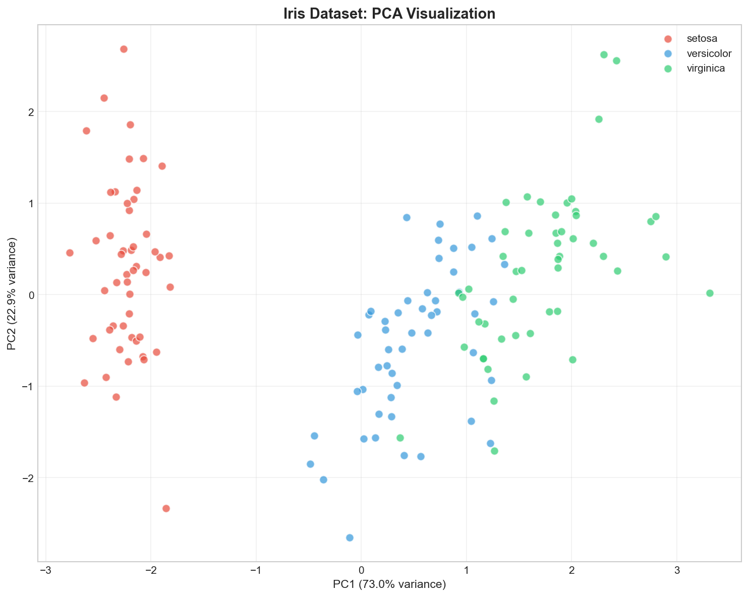
Visualizing in 2D

 1
 2
 3
 4
 5
 6
 7
 8
 9
10
11
12
13
14
15
16
17
18
19

# Plot first two principal components
fig, ax = plt.subplots(figsize=(10, 8))
colors = ['#e74c3c', '#3498db', '#2ecc71']
target_names = iris.target_names

for i, (color, name) in enumerate(zip(colors, target_names)):
    mask = y == i
    ax.scatter(X_pca[mask, 0], X_pca[mask, 1], 
               c=color, alpha=0.7, s=60, label=name, edgecolors='white')

ax.set_xlabel(f'PC1 ({pca.explained_variance_ratio_[0]:.1%} variance)', fontsize=11)
ax.set_ylabel(f'PC2 ({pca.explained_variance_ratio_[1]:.1%} variance)', fontsize=11)
ax.set_title('Iris Dataset: PCA Visualization', fontsize=14, fontweight='bold')
ax.legend()
ax.grid(True, alpha=0.3)

plt.tight_layout()
plt.savefig('assets/pca_iris_2d.png', dpi=150)
plt.show()

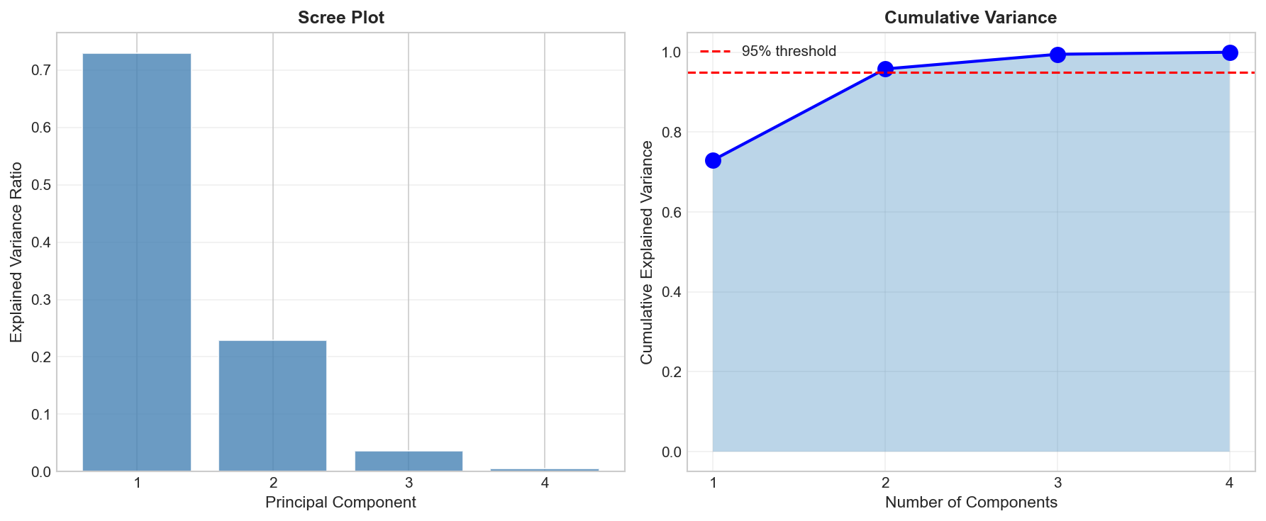
Scree Plot and Choosing Components

 1
 2
 3
 4
 5
 6
 7
 8
 9
10
11
12
13
14
15
16
17
18
19
20
21
22
23
24
25
26
27
28

fig, axes = plt.subplots(1, 2, figsize=(12, 5))

# Individual variance
axes[0].bar(range(1, 5), pca.explained_variance_ratio_, 
            color='steelblue', alpha=0.8, edgecolor='white')
axes[0].set_xlabel('Principal Component', fontsize=11)
axes[0].set_ylabel('Explained Variance Ratio', fontsize=11)
axes[0].set_title('Scree Plot', fontsize=12, fontweight='bold')
axes[0].set_xticks(range(1, 5))
axes[0].grid(True, alpha=0.3, axis='y')

# Cumulative variance
cumsum = np.cumsum(pca.explained_variance_ratio_)
axes[1].plot(range(1, 5), cumsum, 'bo-', linewidth=2, markersize=10)
axes[1].axhline(y=0.95, color='r', linestyle='--', label='95% threshold')
axes[1].fill_between(range(1, 5), cumsum, alpha=0.3)
axes[1].set_xlabel('Number of Components', fontsize=11)
axes[1].set_ylabel('Cumulative Explained Variance', fontsize=11)
axes[1].set_title('Cumulative Variance', fontsize=12, fontweight='bold')
axes[1].set_xticks(range(1, 5))
axes[1].legend()
axes[1].grid(True, alpha=0.3)

plt.tight_layout()
plt.savefig('assets/explained_variance.png', dpi=150)
plt.show()

print(f"\n💡 Recommendation: Use 2 components for 95.8% variance")

How to read this plot?

• The Elbow: Look for where the blue line levels off (after PC2).
• The Threshold: We want >95% total variance. PC1 (73%) + PC2 (23%) = 96%. Sufficient!

Understanding Principal Components

1
2
3
4
5
6
7
8
9

# Show component loadings
components_df = np.round(pca.components_, 3)

print("\n📐 Principal Component Loadings:")
print("=" * 50)
for i, component in enumerate(components_df):
    print(f"\nPC{i+1}:")
    for feature, loading in zip(iris.feature_names, component):
        print(f"  {feature:20s}: {loading:+.3f}")

Output:

 1
 2
 3
 4
 5
 6
 7
 8
 9
10
11
12
13
14
15
16
17
18
19
20
21
22
23
24
25
26

📐 Principal Component Loadings:
==================================================

PC1:
  sepal length (cm)   : +0.521
  sepal width (cm)    : -0.269
  petal length (cm)   : +0.580
  petal width (cm)    : +0.565

PC2:
  sepal length (cm)   : +0.377
  sepal width (cm)    : +0.923
  petal length (cm)   : +0.024
  petal width (cm)    : +0.067

PC3:
  sepal length (cm)   : +0.720
  sepal width (cm)    : -0.244
  petal length (cm)   : -0.142
  petal width (cm)    : -0.634

PC4:
  sepal length (cm)   : -0.261
  sepal width (cm)    : +0.124
  petal length (cm)   : +0.801
  petal width (cm)    : -0.524

PCA for Preprocessing

 1
 2
 3
 4
 5
 6
 7
 8
 9
10
11
12
13

from sklearn.linear_model import LogisticRegression
from sklearn.model_selection import cross_val_score

# Compare: full features vs PCA-reduced
scores_full = cross_val_score(LogisticRegression(max_iter=200), X_scaled, y, cv=5)
scores_pca2 = cross_val_score(LogisticRegression(max_iter=200), X_pca[:, :2], y, cv=5)

print("=" * 50)
print("PCA AS PREPROCESSING")
print("=" * 50)
print(f"\n📊 Full features (4D): {scores_full.mean():.3f} ± {scores_full.std():.3f}")
print(f"📊 PCA 2D:             {scores_pca2.mean():.3f} ± {scores_pca2.std():.3f}")
print(f"\n💡 Near-identical performance with half the dimensions!")

Output:

1
2
3
4
5
6
7
8

==================================================
PCA AS PREPROCESSING
==================================================

📊 Full features (4D): 0.960 ± 0.039
📊 PCA 2D:             0.913 ± 0.054

💡 Near-identical performance with half the dimensions!

Interpreting the Results

• Full Features (4D): The model has access to every precise measurement.
• PCA (2D): The model is seeing a “flat photo” of the data.
• Result: Even though we flattened 4 dimensions into 2, we kept the important structure (95% variance), so the model still works perfectly. This proves the other 2 dimensions were mostly noise or redundancy!

Deep Dive

When PCA Works Well

When PCA Fails

PCA limitations:

1. Non-linear structure: PCA only finds linear projections
2. Important variance ≠ useful variance: Variance may not correlate with class separation
3. Interpretability: Components are combinations of features
4. Scale sensitivity: Features must be standardized first!

PCA Variants

Frequently Asked Questions

Q1: Should I always scale before PCA?

Yes! PCA maximizes variance, so high-variance features dominate without scaling. Always use StandardScaler first.

Q2: Can PCA be used for feature selection?

Not directly — PCA creates new features (components), not selects original ones. For selection, use methods like L1 regularization or recursive feature elimination.

Q3: What if I need more than 95% variance?

The threshold is problem-dependent:

• Visualization: 2-3 components often enough
• Preprocessing: 90-99% depending on downstream task
• Compression: Balance quality vs. storage

Summary

References

• sklearn PCA Documentation
• Jolliffe, I.T. (2002). “Principal Component Analysis”
• “The Elements of Statistical Learning” by Hastie et al. - Chapter 14.5