Learning Objectives

After reading this post, you will be able to:

• Understand the difference between agglomerative and divisive clustering
• Master the four main linkage methods and when to use each
• Read and interpret dendrograms for data exploration
• Choose the optimal number of clusters using dendrogram analysis

Theory

The Intuition: The Digital Librarian

Imagine you have a messy hard drive with thousands of random files (images, documents, code). You don’t just dump them into 3 arbitrary buckets. Instead, you organize them hierarchically:

1. Files go into specific sub-folders (e.g., “vacation_photos”).
2. Sub-folders go into broader categories (e.g., “Photos”).
3. Categories go into the root drive (e.g., “D: Drive”).

This is exactly what Hierarchical Clustering does. It organizes your data into a tree of nested clusters, giving you a complete map of how data points relate to each other at different levels of granularity.

What is Hierarchical Clustering?

Unlike K-Means, which forces you to choose $K$ clusters upfront (flat clustering), Hierarchical Clustering builds a tree structure (Dendrogram) that preserves the relationships between all points.

Two main approaches exist:

Agglomerative Clustering Algorithm

The algorithm proceeds as follows:

1. Initialize: Each data point is its own cluster ($N$ clusters)
2. Find closest pair: Identify the two most similar clusters
3. Merge: Combine them into a single cluster
4. Repeat: Until only one cluster remains
5. Output: A hierarchical tree (dendrogram)

Linkage: The Rules of Organization

The librarian needs a rule to decide which folders to merge next. How do we measure distance between clusters?

Different linkage methods define cluster distance differently:

Mathematical Definitions

For clusters $A$ and $B$:

Single linkage: $$d(A, B) = \min_{a \in A, b \in B} |a - b|$$

Complete linkage: $$d(A, B) = \max_{a \in A, b \in B} |a - b|$$

Average linkage: $$d(A, B) = \frac{1}{|A||B|} \sum_{a \in A} \sum_{b \in B} |a - b|$$

Ward’s method: $$d(A, B) = \sqrt{\frac{2|A||B|}{|A|+|B|}} |\mu_A - \mu_B|$$

The Dendrogram: The Map of Your Data

A dendrogram is a tree diagram showing the full history of merges or splits. It is essentially the “directory tree” of your data.

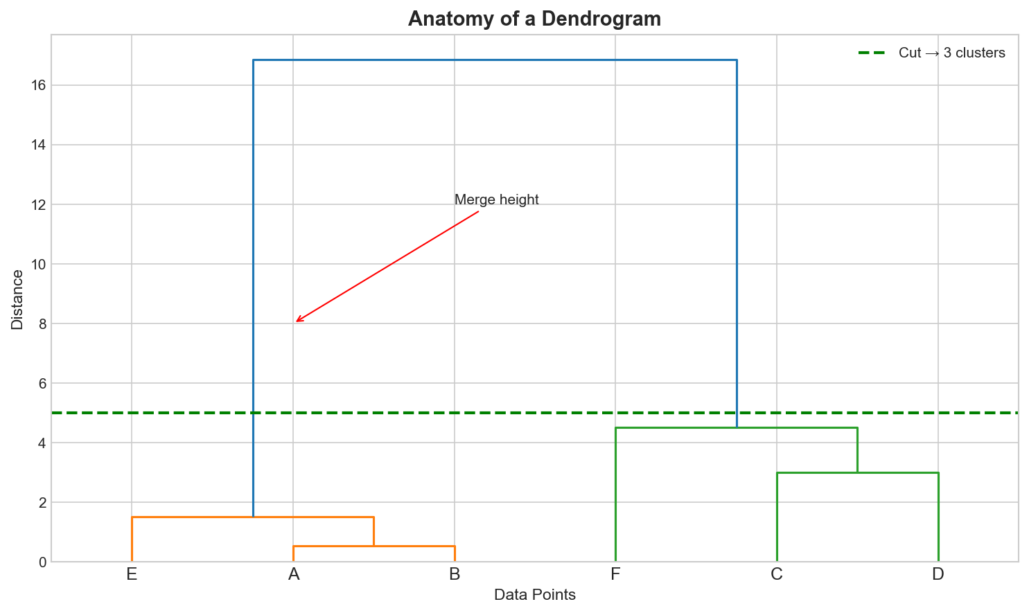
Key elements:

• Leaves: Individual data points (bottom)
• Vertical lines: Clusters being merged
• Height: Distance at which merge occurs
• Horizontal cut: Determines number of clusters

To get $K$ clusters, draw a horizontal line that crosses exactly $K$ vertical lines.

Choosing the Number of Clusters

Unlike K-Means, hierarchical clustering doesn’t require specifying $K$ upfront. Two approaches:

1. Visual inspection of dendrogram

• Look for large gaps in merge heights
• Cut where there’s the biggest “jump”

2. Inconsistency coefficient

• Compare each merge height to previous merges
• High inconsistency suggests a natural boundary

Code Practice

Now, let’s hand over the job to the algorithm. We will let Python act as the digital librarian, automatically sorting our raw data into a structured hierarchy.

Agglomerative Clustering with sklearn

 1
 2
 3
 4
 5
 6
 7
 8
 9
10
11
12
13
14
15
16
17
18
19
20

import numpy as np
import matplotlib.pyplot as plt
from sklearn.datasets import make_blobs
from sklearn.cluster import AgglomerativeClustering
from scipy.cluster.hierarchy import dendrogram, linkage

# Generate sample data
np.random.seed(42)
X, y_true = make_blobs(n_samples=50, centers=3, cluster_std=0.7, random_state=42)

# Perform agglomerative clustering
# linkage='ward': Minimizes variance significantly (good for spherical clusters)
agg = AgglomerativeClustering(n_clusters=3, linkage='ward')
labels = agg.fit_predict(X)

print("=" * 50)
print("AGGLOMERATIVE CLUSTERING RESULTS")
print("=" * 50)
print(f"\n📊 Cluster sizes: {np.bincount(labels)}")
print(f"🔗 Linkage method: Ward")

Output:

1
2
3
4
5
6

==================================================
AGGLOMERATIVE CLUSTERING RESULTS
==================================================

📊 Cluster sizes: [17 16 17]
🔗 Linkage method: Ward

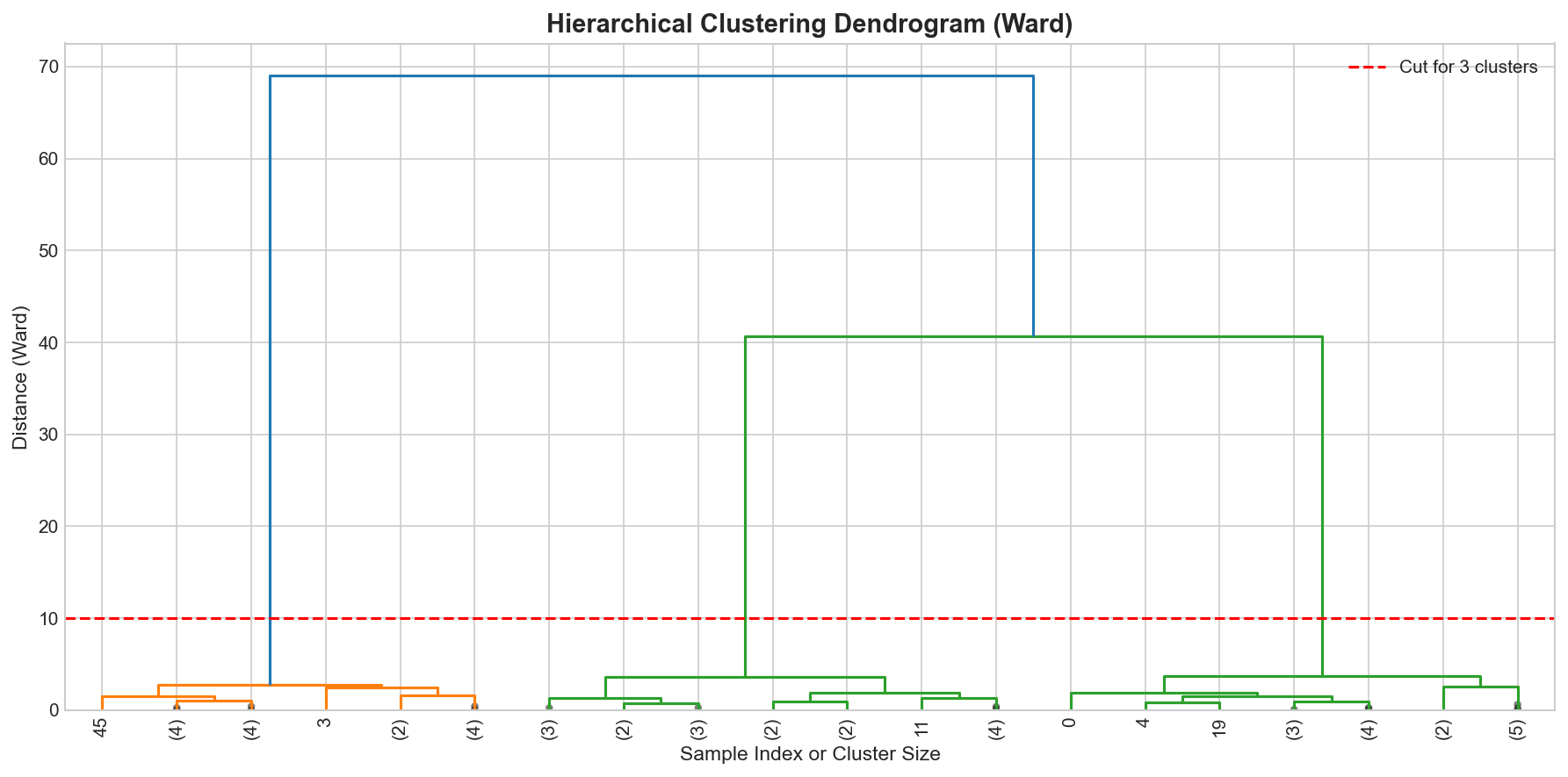
Creating and Interpreting Dendrograms

 1
 2
 3
 4
 5
 6
 7
 8
 9
10
11
12
13
14
15
16
17
18
19
20
21
22
23
24
25
26
27

from scipy.cluster.hierarchy import dendrogram, linkage, fcluster

# Compute linkage matrix
Z = linkage(X, method='ward')

# Create dendrogram
fig, ax = plt.subplots(figsize=(12, 6))
dendrogram(Z, 
           truncate_mode='lastp',  # Simplify the plot: only show the last p merged clusters
           p=20,                    # Show only the top 20 merges (cleaner visualization)
           leaf_rotation=90,
           leaf_font_size=10,
           show_contracted=True)    # Show small dots for contracted clusters

ax.set_title('Hierarchical Clustering Dendrogram (Ward)', fontsize=14, fontweight='bold')
ax.set_xlabel('Sample Index or Cluster Size', fontsize=11)
ax.set_ylabel('Distance (Ward)', fontsize=11)
ax.axhline(y=10, color='r', linestyle='--', label='Cut for 3 clusters')
ax.legend()

plt.tight_layout()
plt.savefig('assets/dendrogram_example.png', dpi=150)
plt.show()

# Get cluster labels by cutting the dendrogram
labels_cut = fcluster(Z, t=3, criterion='maxclust')
print(f"\n📊 Labels from dendrogram cut: {np.bincount(labels_cut)[1:]}")

Output:

1

📊 Labels from dendrogram cut: [16 17 17]

Comparing Linkage Methods

 1
 2
 3
 4
 5
 6
 7
 8
 9
10
11
12
13
14
15
16
17
18
19
20
21
22
23
24
25
26
27
28
29
30

from sklearn.datasets import make_moons

# Generate non-spherical data
X_moons, y_moons = make_moons(n_samples=200, noise=0.05, random_state=42)

# Compare linkage methods
linkage_methods = ['single', 'complete', 'average', 'ward']

fig, axes = plt.subplots(2, 2, figsize=(12, 10))
axes = axes.flatten()

colors = ['#e74c3c', '#3498db']

for ax, method in zip(axes, linkage_methods):
    # We try 2 clusters for everything to see how they split the "moons"
    agg = AgglomerativeClustering(n_clusters=2, linkage=method)
    labels = agg.fit_predict(X_moons)
    
    for i in range(2):
        mask = labels == i
        ax.scatter(X_moons[mask, 0], X_moons[mask, 1], 
                   c=colors[i], alpha=0.6, s=40, edgecolors='white')
    
    ax.set_title(f'{method.capitalize()} Linkage', fontsize=12, fontweight='bold')
    ax.grid(True, alpha=0.3)

plt.suptitle('Linkage Methods on Moon-Shaped Data', fontsize=14, fontweight='bold')
plt.tight_layout()
plt.savefig('assets/linkage_comparison.png', dpi=150)
plt.show()

When to Use Which Linkage?

 1
 2
 3
 4
 5
 6
 7
 8
 9
10
11

from sklearn.metrics import adjusted_rand_score

print("=" * 50)
print("LINKAGE METHOD COMPARISON (Moons Data)")
print("=" * 50)

for method in linkage_methods:
    agg = AgglomerativeClustering(n_clusters=2, linkage=method)
    labels = agg.fit_predict(X_moons)
    ari = adjusted_rand_score(y_moons, labels)
    print(f"{method.capitalize():10} Linkage: ARI = {ari:.4f}")

Output:

1
2
3
4
5
6
7

==================================================
LINKAGE METHOD COMPARISON (Moons Data)
==================================================
Single     Linkage: ARI = 1.0000
Complete   Linkage: ARI = 0.4461
Average    Linkage: ARI = 0.4464
Ward       Linkage: ARI = 0.4464

Interpreting the Results

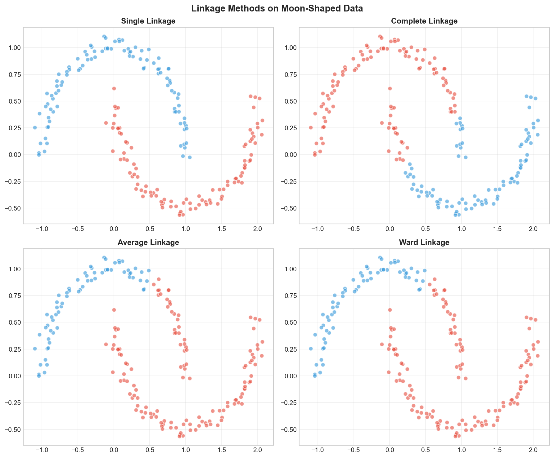
Notice the stark difference!

• Single Linkage (“The Optimist”) achieved a perfect score (ARI=1.0) because it could “chain” along the curved moon shapes. It only needs one pair of close points to merge clusters.
• Ward (“The Architect”) failed (ARI ~0.45) because it tries to minimize variance, forcing the data into spherical (ball-like) shapes. It cut right through the crescents!

Decision Guide

So, which one should you choose?

Deep Dive

Hierarchical vs K-Means

Computational Complexity

Frequently Asked Questions

Q1: When should I use hierarchical clustering over K-Means?

Use hierarchical clustering when:

• You don’t know how many clusters exist
• You want to explore data structure at multiple scales
• You need a dendrogram for interpretation
• Dataset is small enough ($N < 10000$)

Q2: Can I use hierarchical clustering with categorical data?

Yes, but you need an appropriate distance metric:

• Hamming distance: Count of differing attributes
• Jaccard distance: For binary/set data
• Gower distance: For mixed data types

Summary

References

• sklearn Hierarchical Clustering
• scipy.cluster.hierarchy Documentation
• Müllner, D. (2011). “Modern hierarchical, agglomerative clustering algorithms”
• “The Elements of Statistical Learning” - Chapter 14.3