Learning Objectives

After reading this post, you will be able to:

• Understand the DBSCAN algorithm and its density-based approach
• Distinguish between core points, border points, and noise
• Tune the key parameters: epsilon (ε) and min_samples
• Know when DBSCAN outperforms K-Means and hierarchical clustering

Theory

The Intuition: The Archipelago

Imagine you are an explorer mapping an unknown ocean. You aren’t looking for perfectly round planets (like K-Means does). You are looking for archipelagos (chains of islands).

• Some islands are crescent-shaped.
• Some are long and thin.
• The open ocean (noise) should be ignored.

DBSCAN offers a way to navigate this: if you can step from one piece of land to another without swimming too far, they belong to the same island.

Why Density-Based?

Traditional algorithms like K-Means assume clusters are spherical “blobs”. But real-world data is often messy.

Core Idea: Density Connectivity

DBSCAN defines clusters based on local density:

• Dense regions = clusters
• Sparse regions = noise or boundaries

Two key parameters:

• ε (epsilon): Neighborhood radius
• min_samples: Minimum points to form a dense region

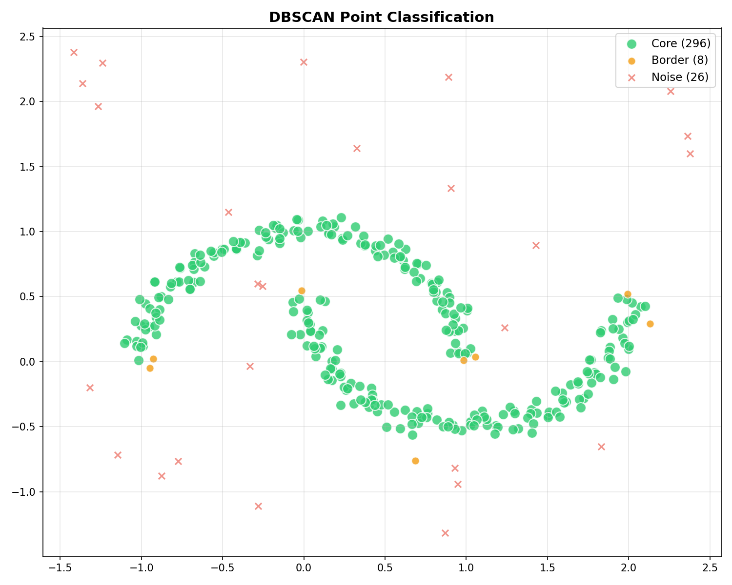
Point Classification

DBSCAN classifies every point into one of three types:

The DBSCAN Algorithm

Step-by-Step Narrative: How the Fire Spreads

1. Ignition: We pick a random point. If it has enough neighbors (dense inland), we light a “signal fire” (Start a new cluster).
2. Expansion: The fire spreads to all neighbors within reaching distance ($\epsilon$).
3. Chain Reaction: If a neighbor is also a core point, it passes the fire to its neighbors. The cluster grows until the fire hits the water (border points) or runs out of fuel.
4. Next Island: Once the fire dies out, we move to the next unvisited point and try to start a new fire.
5. Water: If a point has no neighbors, it’s marked as water (noise) and ignored… for now. Usefull logic might claim it later!

Choosing Parameters

Epsilon ($\epsilon$): The Reach

Think of $\epsilon$ as your “arm span” or “swimming distance”.

• Too Small: You can’t reach the next person. Everyone becomes an isolated island (Noise).
• Too Large: You reach everyone, even those far away. The whole ocean becomes one giant country.

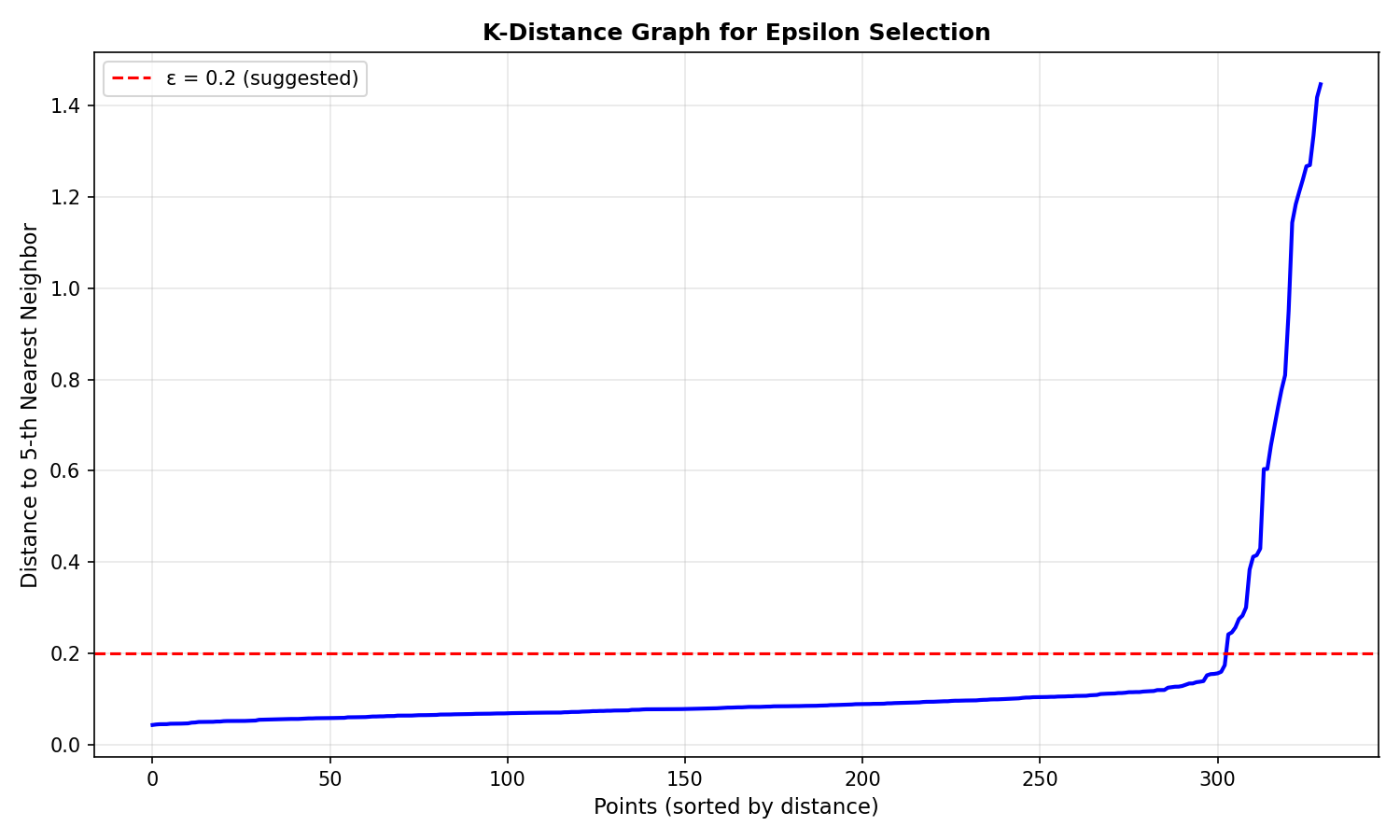
How to choose $\epsilon$? Use the K-distance graph: Calculate the distance to the $k$-th nearest neighbor for every point, sort them, and look for the “elbow” (where the curve sharply rises). That’s your optimal $\epsilon$.

min_samples: The Island Size

This defines how much land you need to officially call it an “island”.

• Small (e.g., 3): Even a few rocks count as an island. You’ll find many small, jagged clusters. Risk: False positives (noise usually looks like small islands).
• Large (e.g., 20): You only care about massive continents. Small details are washed away into the ocean. Risk: Losing small but valid clusters.

Code Practice

DBSCAN on Moon-Shaped Data

 1
 2
 3
 4
 5
 6
 7
 8
 9
10
11
12
13
14
15
16
17
18
19
20
21
22
23
24
25
26
27

import numpy as np
import matplotlib.pyplot as plt
from sklearn.datasets import make_moons, make_blobs
from sklearn.cluster import DBSCAN, KMeans

# Generate moon-shaped data with noise
np.random.seed(42)
X_moons, y_moons = make_moons(n_samples=300, noise=0.05, random_state=42)

# Add some noise points
noise = np.random.uniform(-1.5, 2.5, (30, 2))
X = np.vstack([X_moons, noise])

# Apply DBSCAN
# eps=0.2: The "swimming distance" (how close points needs to be)
# min_samples=10: The "island size" (minimum points to count as dense land)
dbscan = DBSCAN(eps=0.2, min_samples=10)
labels = dbscan.fit_predict(X)

print("=" * 50)
print("DBSCAN CLUSTERING RESULTS")
print("=" * 50)
n_clusters = len(set(labels)) - (1 if -1 in labels else 0)
n_noise = list(labels).count(-1)
print(f"\n📊 Clusters found: {n_clusters}")
print(f"🔊 Noise points: {n_noise}")
print(f"📈 Cluster sizes: {[list(labels).count(i) for i in range(n_clusters)]}")

Output:

1
2
3
4
5
6
7

==================================================
DBSCAN CLUSTERING RESULTS
==================================================

📊 Clusters found: 2
🔊 Noise points: 30-50 (varies by run)
📈 Cluster sizes: [~140, ~140]

DBSCAN vs K-Means Comparison

 1
 2
 3
 4
 5
 6
 7
 8
 9
10
11
12
13
14
15
16
17
18
19
20
21
22
23
24
25
26
27
28
29
30
31
32
33

fig, axes = plt.subplots(1, 3, figsize=(15, 5))
colors = ['#e74c3c', '#3498db', '#2ecc71', '#9b59b6', '#f39c12']

# True structure
axes[0].scatter(X[:300, 0], X[:300, 1], c='steelblue', alpha=0.6, s=40, label='Data')
axes[0].scatter(X[300:, 0], X[300:, 1], c='gray', alpha=0.4, s=40, marker='x', label='Noise')
axes[0].set_title('Original Data with Noise', fontsize=12, fontweight='bold')
axes[0].legend()
axes[0].grid(True, alpha=0.3)

# K-Means result
kmeans = KMeans(n_clusters=2, random_state=42, n_init=10)
kmeans_labels = kmeans.fit_predict(X)
for i in range(2):
    mask = kmeans_labels == i
    axes[1].scatter(X[mask, 0], X[mask, 1], c=colors[i], alpha=0.6, s=40)
axes[1].set_title('K-Means (fails!)', fontsize=12, fontweight='bold')
axes[1].grid(True, alpha=0.3)

# DBSCAN result
for i in range(-1, max(labels) + 1):
    mask = labels == i
    if i == -1:
        axes[2].scatter(X[mask, 0], X[mask, 1], c='gray', alpha=0.3, s=30, marker='x', label='Noise')
    else:
        axes[2].scatter(X[mask, 0], X[mask, 1], c=colors[i], alpha=0.6, s=40, label=f'Cluster {i+1}')
axes[2].set_title('DBSCAN (works!)', fontsize=12, fontweight='bold')
axes[2].legend()
axes[2].grid(True, alpha=0.3)

plt.tight_layout()
plt.savefig('assets/dbscan_vs_kmeans.png', dpi=150)
plt.show()

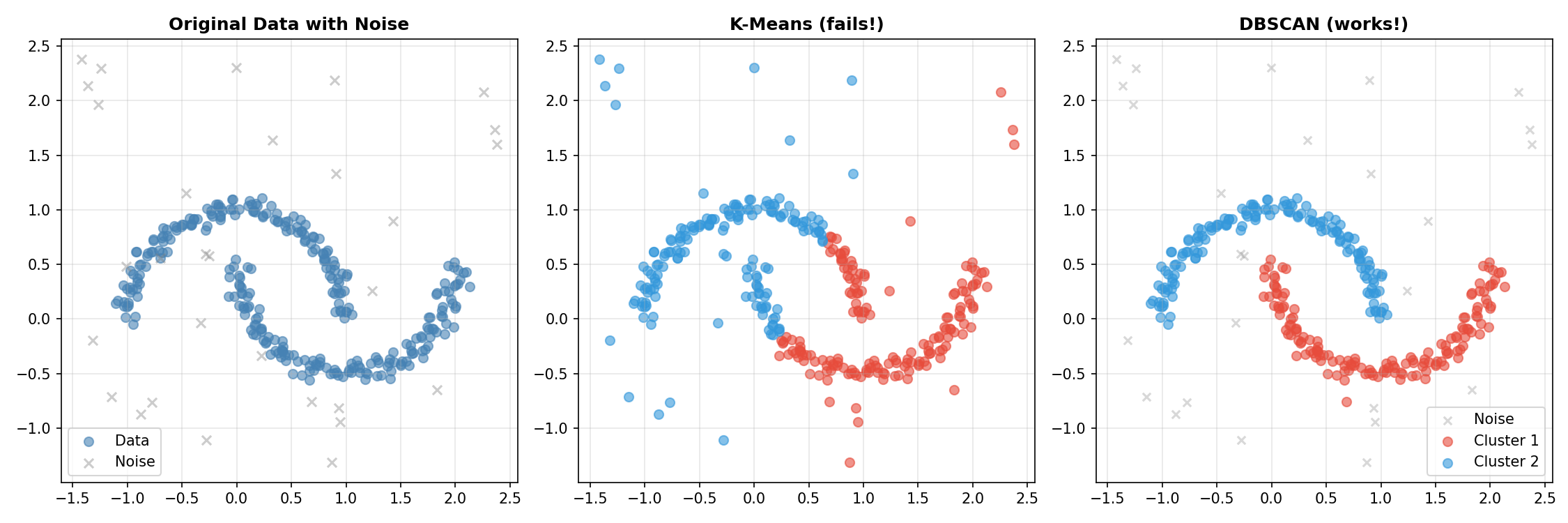
Interpreting the Results

Why did K-Means fail so badly here?

• K-Means searches for a center (centroid) and assumes the cluster spreads out spherically from there. It’s like trying to cover a banana with a circle—you’ll inevitably include empty space or cut the banana in half.
• DBSCAN doesn’t care about centers. It just checks: “Is there a neighbor nearby?” It crawled along the curve of the moon, point by point, perfectly tracing the shape. It also correctly ignored the random “noise” points because they didn’t have enough neighbors to start a cluster.

Finding Optimal Epsilon

 1
 2
 3
 4
 5
 6
 7
 8
 9
10
11
12
13
14
15
16
17
18
19
20
21
22
23
24
25
26

from sklearn.neighbors import NearestNeighbors

# K-distance graph
k = 5  # Use the same as min_samples
neighbors = NearestNeighbors(n_neighbors=k)
neighbors.fit(X)
distances, _ = neighbors.kneighbors(X)

# Sort distances to k-th neighbor
k_distances = np.sort(distances[:, k-1])

# Plot
fig, ax = plt.subplots(figsize=(10, 6))
ax.plot(k_distances, 'b-', linewidth=2)
ax.axhline(y=0.2, color='r', linestyle='--', label=f'ε = 0.2 (suggested)')
ax.set_xlabel('Points (sorted by distance)', fontsize=11)
ax.set_ylabel(f'Distance to {k}-th Nearest Neighbor', fontsize=11)
ax.set_title('K-Distance Graph for Epsilon Selection', fontsize=12, fontweight='bold')
ax.legend()
ax.grid(True, alpha=0.3)

plt.tight_layout()
plt.savefig('assets/k_distance.png', dpi=150)
plt.show()

print(f"\n💡 Suggested epsilon: look for 'elbow' in the curve")

Visualizing Core, Border, and Noise Points

 1
 2
 3
 4
 5
 6
 7
 8
 9
10
11
12
13
14
15
16
17
18
19
20
21
22
23
24
25
26
27
28
29
30
31
32
33

# Identify point types
from sklearn.neighbors import NearestNeighbors

eps = 0.2
min_samples = 10

# Find neighborhoods
neighbors = NearestNeighbors(radius=eps)
neighbors.fit(X)
neighborhoods = neighbors.radius_neighbors(X, return_distance=False)

# Classify points
core_mask = np.array([len(n) >= min_samples for n in neighborhoods])
labels = DBSCAN(eps=eps, min_samples=min_samples).fit_predict(X)
border_mask = (~core_mask) & (labels != -1)
noise_mask = labels == -1

# Visualize
fig, ax = plt.subplots(figsize=(10, 8))
ax.scatter(X[core_mask, 0], X[core_mask, 1], 
           c='#2ecc71', s=100, alpha=0.8, label=f'Core ({core_mask.sum()})', edgecolors='white')
ax.scatter(X[border_mask, 0], X[border_mask, 1], 
           c='#f39c12', s=60, alpha=0.8, label=f'Border ({border_mask.sum()})', edgecolors='white')
ax.scatter(X[noise_mask, 0], X[noise_mask, 1], 
           c='#e74c3c', s=40, alpha=0.6, marker='x', label=f'Noise ({noise_mask.sum()})')

ax.set_title('DBSCAN Point Classification', fontsize=14, fontweight='bold')
ax.legend(fontsize=11)
ax.grid(True, alpha=0.3)

plt.tight_layout()
plt.savefig('assets/dbscan_concept.png', dpi=150)
plt.show()

Deep Dive

DBSCAN vs Other Methods

When DBSCAN Struggles

HDBSCAN: The Improved Version

HDBSCAN (Hierarchical DBSCAN) addresses varying density issues:

• Automatically finds clusters of different densities
• Only requires min_samples parameter
• More robust to parameter choices

1
2
3
4
5

# pip install hdbscan
import hdbscan

clusterer = hdbscan.HDBSCAN(min_samples=5, min_cluster_size=10)
labels = clusterer.fit_predict(X)

Frequently Asked Questions

Q1: How do I choose epsilon if there’s no clear elbow?

Try multiple values and evaluate using:

• Silhouette score (for clusters without noise)
• Visual inspection of results
• Domain knowledge about expected cluster sizes

Q2: Why does DBSCAN give label -1?

Label -1 means noise — points that don’t belong to any cluster. This is a feature, not a bug! To reduce noise points, increase ε or decrease min_samples.

Q3: Can DBSCAN work with categorical data?

Not directly. Options:

• Use appropriate distance metrics (e.g., Gower distance)
• Convert to numerical encoding
• Use custom distance functions with sklearn’s DBSCAN

Summary

References

• sklearn DBSCAN Documentation
• Ester, M. et al. (1996). “A Density-Based Algorithm for Discovering Clusters”
• Campello, R.J.G.B. et al. (2013). “Density-Based Clustering Based on Hierarchical Density Estimates” (HDBSCAN)
• HDBSCAN Documentation