Unlock the power of clustering. Master Lloyd's Algorithm from scratch, visualize the iterative 'Assignment-Update' loop, and solve the 'How many clusters?' dilemma with the Elbow Method.
Learning Objectives
After reading this post, you will be able to:
Understand the K-Means algorithm step-by-step
Implement Lloyd’s algorithm from scratch
Use the elbow method to choose the optimal number of clusters
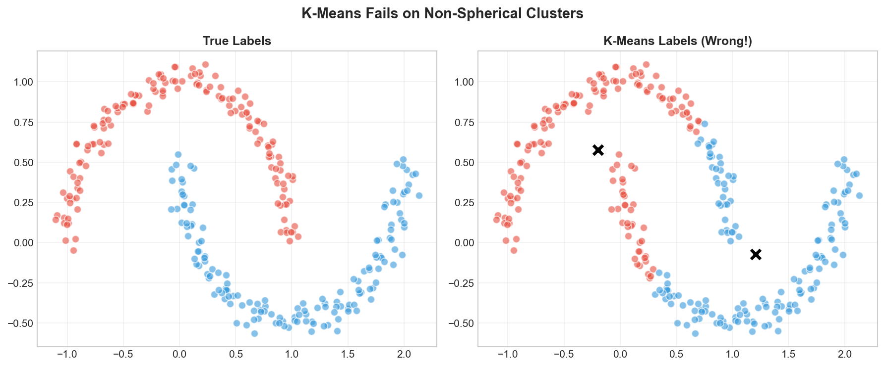
Know when K-Means works well and when it fails
Theory
The Intuition: The Delivery Problem
Imagine you are a logistics manager for a city and you want to open K delivery centers. Your goal is simple: maximize efficiency by ensuring that the average travel time for all customers to their nearest center is minimized.
Initialize: You place $K$ centers at random locations.
Assign: You assign every customer to their nearest center.
Update: You realize the centers aren’t optimal, so you move each center to the “middle” (centroid) of its assigned customers.
Repeat: You keep moving the centers and re-assigning customers until the centers stop moving.
This is exactly how K-Means works. It is an iterative algorithm that tries to find the best “centers” for your data.
What is K-Means?
K-Means partitions data into $k$ distinct, non-overlapping groups (clusters). The algorithm assigns each data point to the cluster with the nearest centroid.
graph LR
subgraph Goal ["K-Means Goal"]
direction LR
A["Data Points"] --> B["K-Means"]
B --> C["K Clusters"]
end
style B fill:#fff9c4
style C fill:#c8e6c9
The K-Means Objective
Formally, K-Means minimizes the sum of squared distances from each point to its assigned centroid:
Convergence guarantee: Lloyd’s algorithm always converges because each step reduces (or maintains) the objective $J$. However, it may converge to a local minimum, not the global optimum.
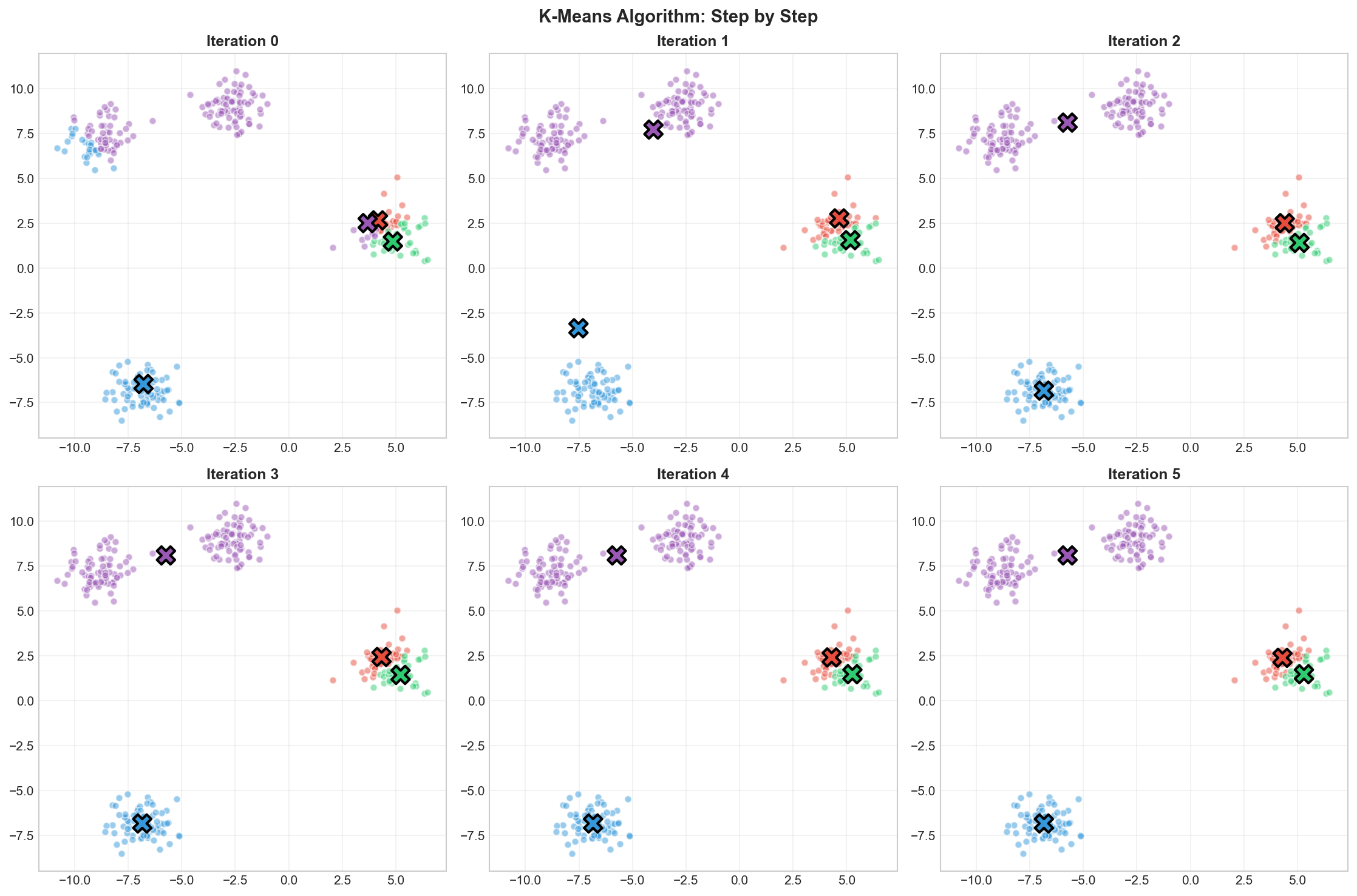
Step-by-Step Example
Let’s trace through K-Means with $K=2$ on simple 2D data:
Iteration 0: Initialize
Randomly select 2 points as initial centroids
Iteration 1: Assign + Update
Assign each point to its nearest centroid
Recompute centroids as the mean of assigned points
Iteration 2+: Repeat
Continue until centroids stabilize
K-Means iterations: random initialization → assignment → update → convergence
Initialization Strategies
The initial centroids strongly affect the final result. Common strategies:
Strategy
Description
Quality
Random
Pick $K$ random points
⚠️ Inconsistent
Random partition
Randomly assign points, then compute centroids
⚠️ Inconsistent
K-Means++
Smart initialization, spread out centroids
✅ Better
Multiple runs
Run algorithm $n$ times, pick best result
✅ Robust
K-Means++ initialization (default in sklearn): Pick the first centroid randomly, then pick subsequent centroids with probability proportional to squared distance from existing centroids. This spreads out initial centroids and typically leads to better results.
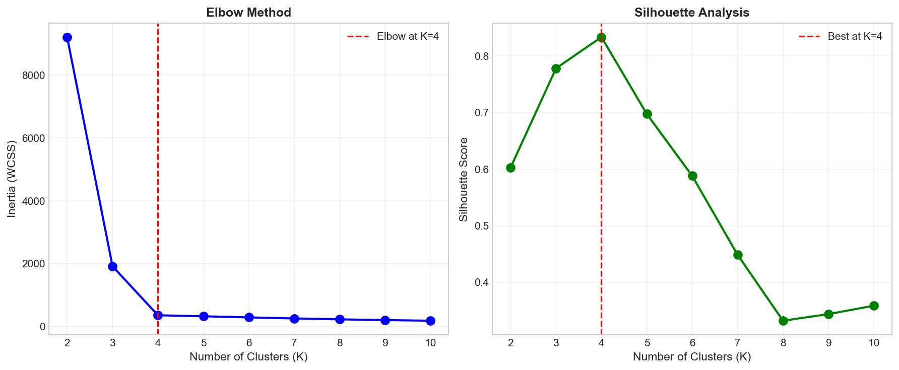
Choosing K: The Elbow Method
A key question: how many clusters should we use?
The elbow method plots inertia (WCSS) against $K$ and looks for an “elbow” — a point where adding more clusters gives diminishing returns.
Elbow method: Look for the 'elbow' where inertia decreases sharply then levels off
Practical Tip:
The “elbow” isn’t always sharp! It’s often subjective. If the elbow is at K=3, but K=4 makes more business sense (e.g., 4 clothing sizes: S, M, L, XL), choose the business logic. Models are tools, not masters.
Silhouette Score
Another approach is the silhouette score, which measures how similar points are to their own cluster vs. other clusters:
$$s(i) = \frac{b(i) - a(i)}{\max(a(i), b(i))}$$
where:
$a(i)$ = mean distance from point $i$ to other points in same cluster
$b(i)$ = mean distance to points in nearest other cluster
$s(i) \in [-1, 1]$: higher is better
Score
Interpretation
$\approx 1$
Well-clustered
$\approx 0$
On cluster boundary
$< 0$
Possibly wrong cluster
Code Practice
Now that we understand the theory and the math, let’s bring it to life with code. We’ll start by building K-Means from scratch to see the mechanics, and then use sklearn for production-ready clustering.
importnumpyasnpimportmatplotlib.pyplotaspltclassKMeansFromScratch:def__init__(self,n_clusters=3,max_iters=100,random_state=42):self.n_clusters=n_clustersself.max_iters=max_itersself.random_state=random_statedeffit(self,X):"""Step-by-step implementation of Lloyd's Algorithm"""np.random.seed(self.random_state)n_samples=X.shape[0]# Step 1: Initialize centroids randomly# We pick k random data points to startrandom_idx=np.random.choice(n_samples,self.n_clusters,replace=False)self.centroids=X[random_idx].copy()self.history=[self.centroids.copy()]foriterationinrange(self.max_iters):# Step 2: Assign points to nearest centroid# We compute distance matrix and find min index for each rowdistances=self._compute_distances(X)self.labels=np.argmin(distances,axis=1)# Step 3: Update centroids# Move centroid to the mean of all points assigned to itnew_centroids=np.array([X[self.labels==k].mean(axis=0)forkinrange(self.n_clusters)])self.history.append(new_centroids.copy())# Check convergence# If centroids didn't move, we are done!ifnp.allclose(self.centroids,new_centroids):print(f"Converged at iteration {iteration+1}")breakself.centroids=new_centroidsreturnselfdef_compute_distances(self,X):"""
Vectorized distance calculation.
Returns a matrix of shape (n_samples, n_clusters)
where [i, k] is the distance from point i to centroid k.
"""distances=np.zeros((X.shape[0],self.n_clusters))fork,centroidinenumerate(self.centroids):# axis=1 means we sum across the columns (x, y coordinates)distances[:,k]=np.linalg.norm(X-centroid,axis=1)returndistancesdefpredict(self,X):"""Assign new points to the nearest cluster"""distances=self._compute_distances(X)returnnp.argmin(distances,axis=1)definertia(self,X):"""Compute within-cluster sum of squares (WCSS)"""distances=self._compute_distances(X)# For each point, take the distance to its assigned centroid (min distance)# Square it, then sum them upreturnnp.sum(np.min(distances,axis=1)**2)# Generate sample datafromsklearn.datasetsimportmake_blobsX,y_true=make_blobs(n_samples=300,centers=4,cluster_std=0.8,random_state=42)# Fit our implementationkmeans=KMeansFromScratch(n_clusters=4,random_state=42)kmeans.fit(X)print(f"\n📊 Final centroids:\n{kmeans.centroids}")print(f"📏 Inertia: {kmeans.inertia(X):.2f}")
# Visualize the algorithm iterationsfig,axes=plt.subplots(2,3,figsize=(15,10))axes=axes.flatten()colors=['#e74c3c','#3498db','#2ecc71','#9b59b6']fori,axinenumerate(axes):ifi>=len(kmeans.history):ax.axis('off')continuecentroids=kmeans.history[i]# Compute labels for this iteration's centroidsdistances=np.array([[np.linalg.norm(x-c)forcincentroids]forxinX])labels=np.argmin(distances,axis=1)# Plot pointsforkinrange(4):mask=labels==kax.scatter(X[mask,0],X[mask,1],c=colors[k],alpha=0.5,s=30)# Plot centroidsax.scatter(centroids[:,0],centroids[:,1],c=colors[:len(centroids)],marker='X',s=200,edgecolors='black',linewidths=2)ax.set_title(f'Iteration {i}',fontsize=12,fontweight='bold')ax.grid(True,alpha=0.3)plt.suptitle('K-Means Algorithm: Step by Step',fontsize=14,fontweight='bold')plt.tight_layout()plt.savefig('assets/kmeans_steps.png',dpi=150)plt.show()
K-Means converges in just 4 iterations on well-separated clusters
Using sklearn K-Means
In practice, use sklearn’s optimized implementation:
fromsklearn.clusterimportKMeansfromsklearn.metricsimportsilhouette_score# Generate dataX,y_true=make_blobs(n_samples=300,centers=4,cluster_std=0.8,random_state=42)# Fit K-Means# n_init=10: Run algorithm 10 times with different random starts and keep the best one.# Crucial to avoid getting stuck in bad local minima!# random_state=42: For reproducibility throughout this tutorial.kmeans=KMeans(n_clusters=4,random_state=42,n_init=10)labels=kmeans.fit_predict(X)print("="*50)print("SKLEARN K-MEANS RESULTS")print("="*50)print(f"\n📊 Cluster sizes: {np.bincount(labels)}")print(f"📏 Inertia: {kmeans.inertia_:.2f}")print(f"📐 Silhouette Score: {silhouette_score(X,labels):.4f}")print(f"🔄 Iterations: {kmeans.n_iter_}")
# Find optimal K using elbow methodinertias=[]silhouettes=[]K_range=range(2,11)forkinK_range:kmeans=KMeans(n_clusters=k,random_state=42,n_init=10)labels=kmeans.fit_predict(X)inertias.append(kmeans.inertia_)silhouettes.append(silhouette_score(X,labels))# Plotfig,axes=plt.subplots(1,2,figsize=(12,5))# Elbow plotaxes[0].plot(K_range,inertias,'bo-',linewidth=2,markersize=8)axes[0].axvline(x=4,color='r',linestyle='--',label='Elbow at K=4')axes[0].set_xlabel('Number of Clusters (K)',fontsize=11)axes[0].set_ylabel('Inertia (WCSS)',fontsize=11)axes[0].set_title('Elbow Method',fontsize=12,fontweight='bold')axes[0].legend()axes[0].grid(True,alpha=0.3)# Silhouette plotaxes[1].plot(K_range,silhouettes,'go-',linewidth=2,markersize=8)axes[1].axvline(x=4,color='r',linestyle='--',label='Best at K=4')axes[1].set_xlabel('Number of Clusters (K)',fontsize=11)axes[1].set_ylabel('Silhouette Score',fontsize=11)axes[1].set_title('Silhouette Analysis',fontsize=12,fontweight='bold')axes[1].legend()axes[1].grid(True,alpha=0.3)plt.tight_layout()plt.savefig('assets/elbow_method.png',dpi=150)plt.show()
Both elbow method and silhouette score suggest K=4 is optimal