Learning Objectives

After reading this post, you will be able to:

• Understand the fundamental differences between supervised and unsupervised learning
• Know the three major categories of unsupervised methods: clustering, dimensionality reduction, and anomaly detection
• Identify appropriate use cases for unsupervised techniques
• Preview the UML series roadmap and what’s coming next

Theory

What is Unsupervised Learning?

Imagine you are an explorer landing on an alien planet. You encounter strange plants and animals you’ve never seen before. There is no guidebook, no teacher, and no labels telling you “this is a tree” or “that is a wolf.”

What do you do?

You start observing. You notice that some creatures have wings and fly (Group A), while others have fins and swim (Group B). You notice that some plants are tall with wood (structure), while others are small and green. You are learning by observation. This is the essence of Unsupervised Learning.

In the Supervised Learning series, every training sample had a label — a “correct answer” provided by a “teacher.” But in the real world, most data is like that alien planet: vast, complex, and completely unlabeled. This is often called Dark Data.

Unsupervised learning discovers hidden patterns, structures, and relationships in this “dark” data without any labels. Instead of learning input-output mappings (like a student preparing for a test), these algorithms find the underlying structure in the data itself (like a scientist discovering natural laws).

Supervised vs Unsupervised: A Comparison

The Explorer’s Toolkit

Just as an explorer uses different tools for different terrains (maps, compasses, drills), we use three main types of unsupervised learning to navigate unknown data:

Clustering: Finding Groups

Clustering partitions data into groups (clusters) where:

• Points within a cluster are similar to each other
• Points in different clusters are dissimilar

Use cases:

• Customer segmentation (group customers by behavior)
• Document categorization (group similar articles)
• Image segmentation (group similar pixels)
• Gene expression analysis (group similar genes)

Dimensionality Reduction: Compressing Information

Dimensionality reduction transforms high-dimensional data into a lower-dimensional representation while preserving important information.

Use cases:

• Visualization (plot 100D data in 2D)
• Feature compression (reduce storage/computation)
• Noise reduction (remove irrelevant dimensions)
• Preprocessing for other ML algorithms

Anomaly Detection: Identifying Outliers

Anomaly detection finds data points that differ significantly from the majority — the “unusual” observations.

Use cases:

• Fraud detection (unusual credit card transactions)
• System monitoring (server failures, network intrusions)
• Quality control (defective products)
• Medical diagnosis (rare diseases)

When to Use Unsupervised Learning

Real-World Applications

Code Practice

Let’s put on our boots. In this section, we will take a raw, unlabeled dataset (Dark Data) and act as the explorer. We’ll attempt to rediscover hidden structure without any guide to help us.

Loading Unlabeled Data

In supervised learning, we always loaded data with labels. Now, let’s see what working with unlabeled data looks like:

 1
 2
 3
 4
 5
 6
 7
 8
 9
10
11
12
13
14
15
16
17
18
19
20
21

import numpy as np
import matplotlib.pyplot as plt
from sklearn.datasets import load_iris

# Load the Iris dataset
iris = load_iris()
X = iris.data  # Features only (sepal/petal lengths/widths)

# ⚠️ CRITICAL: In unsupervised learning, we DO NOT use the target (y labels)
# We pretend they don't exist and let the data speak for itself.
# y = iris.target  <-- We ignore this!

feature_names = iris.feature_names

print("=" * 50)
print("UNLABELED DATA EXPLORATION")
print("=" * 50)
print(f"\n📊 Dataset shape: {X.shape}")
print(f"📐 Features: {feature_names}")
print(f"\n🔢 Sample data (first 5 rows):")
print(X[:5])

Output:

 1
 2
 3
 4
 5
 6
 7
 8
 9
10
11
12
13

==================================================
UNLABELED DATA EXPLORATION
==================================================

📊 Dataset shape: (150, 4)
📐 Features: ['sepal length (cm)', 'sepal width (cm)', 'petal length (cm)', 'petal width (cm)']

🔢 Sample data (first 5 rows):
[[5.1 3.5 1.4 0.2]
 [4.9 3.  1.4 0.2]
 [4.7 3.2 1.3 0.2]
 [4.6 3.1 1.5 0.2]
 [5.  3.6 1.4 0.2]]

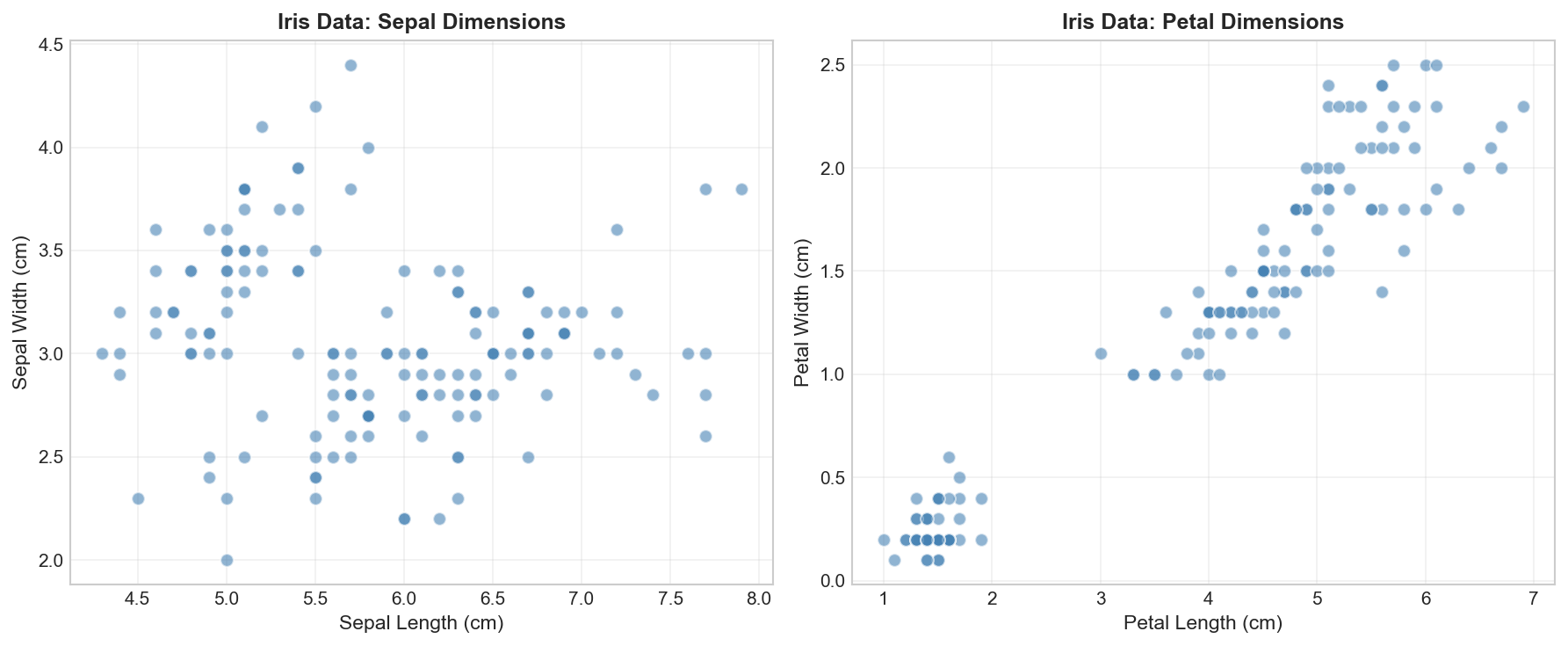
Visualizing Unlabeled Data

Before applying any algorithm, let’s visualize our data to see if natural groupings exist:

 1
 2
 3
 4
 5
 6
 7
 8
 9
10
11
12
13
14
15
16
17
18
19
20

# Visualize data using two features
fig, axes = plt.subplots(1, 2, figsize=(12, 5))

# Plot 1: Sepal dimensions
axes[0].scatter(X[:, 0], X[:, 1], c='steelblue', alpha=0.6, s=50)
axes[0].set_xlabel('Sepal Length (cm)')
axes[0].set_ylabel('Sepal Width (cm)')
axes[0].set_title('Iris Data: Sepal Dimensions')
axes[0].grid(True, alpha=0.3)

# Plot 2: Petal dimensions
axes[1].scatter(X[:, 2], X[:, 3], c='steelblue', alpha=0.6, s=50)
axes[1].set_xlabel('Petal Length (cm)')
axes[1].set_ylabel('Petal Width (cm)')
axes[1].set_title('Iris Data: Petal Dimensions')
axes[1].grid(True, alpha=0.3)

plt.tight_layout()
plt.savefig('assets/unlabeled_data.png', dpi=150)
plt.show()

Looking at the petal dimensions plot, you might already notice some natural clusters. This is exactly what clustering algorithms will help us find!

Preview: K-Means Clustering

Let’s get a sneak peek of what clustering can do. We’ll cover K-Means in detail in the next post, but here’s a quick demo:

 1
 2
 3
 4
 5
 6
 7
 8
 9
10
11
12
13
14
15
16
17
18
19
20
21
22
23
24
25
26
27
28
29
30
31
32
33
34
35
36
37
38
39
40
41
42
43
44
45
46
47
48
49
50

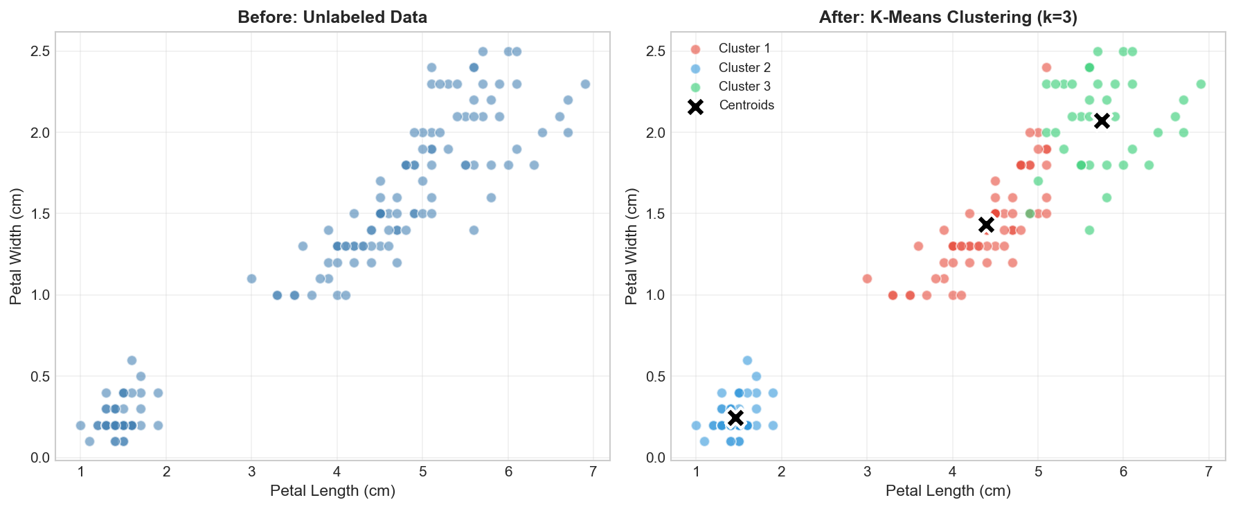
from sklearn.cluster import KMeans

# Apply K-Means clustering
# n_clusters=3: We (the humans) know there are 3 species, but in real life, 
#               you might need to use the 'Elbow Method' to find this number.
# random_state=42: Ensures reproducible results.
# n_init=10: Run the algorithm 10 times with different starting points 
#            to avoid getting stuck in bad local situations.
kmeans = KMeans(n_clusters=3, random_state=42, n_init=10)

# The algorithm learns the structure (fit) and assigns labels (predict)
clusters = kmeans.fit_predict(X)

# Visualize the clustering result
fig, axes = plt.subplots(1, 2, figsize=(12, 5))

# Original data (no labels)
axes[0].scatter(X[:, 2], X[:, 3], c='steelblue', alpha=0.6, s=50)
axes[0].set_xlabel('Petal Length (cm)')
axes[0].set_ylabel('Petal Width (cm)')
axes[0].set_title('Before: Unlabeled Data')
axes[0].grid(True, alpha=0.3)

# Clustered data
colors = ['#e74c3c', '#3498db', '#2ecc71']
for i in range(3):
    mask = clusters == i
    axes[1].scatter(X[mask, 2], X[mask, 3], 
                    c=colors[i], alpha=0.6, s=50, 
                    label=f'Cluster {i+1}')

# Plot cluster centers
centers = kmeans.cluster_centers_
axes[1].scatter(centers[:, 2], centers[:, 3], 
                c='black', marker='X', s=200, 
                edgecolors='white', linewidths=2,
                label='Centroids')

axes[1].set_xlabel('Petal Length (cm)')
axes[1].set_ylabel('Petal Width (cm)')
axes[1].set_title('After: K-Means Clustering (k=3)')
axes[1].legend()
axes[1].grid(True, alpha=0.3)

plt.tight_layout()
plt.savefig('assets/kmeans_preview.png', dpi=150)
plt.show()

print(f"\n📊 Clustering Results:")
print(f"   Cluster sizes: {np.bincount(clusters)}")

Output:

1
2

📊 Clustering Results:
   Cluster sizes: [62 50 38]

Comparing with True Labels (Cheating a Little)

Let’s peek at how well our unsupervised clustering matches the true labels:

 1
 2
 3
 4
 5
 6
 7
 8
 9
10
11
12
13
14
15
16
17
18
19
20
21

from sklearn.metrics import adjusted_rand_score, normalized_mutual_info_score

# True labels (we pretend we didn't have these!)
y_true = iris.target

# Evaluate clustering quality
# Adjusted Rand Index (ARI): Measures similarity between true and predicted labels.
# 0.0 = Random labeling
# 1.0 = Perfect match
ari = adjusted_rand_score(y_true, clusters)

# Normalized Mutual Information (NMI): Just another way to measure agreement.
nmi = normalized_mutual_info_score(y_true, clusters)

print("=" * 50)
print("CLUSTERING EVALUATION (using hidden labels)")
print("=" * 50)
print(f"\n📊 Adjusted Rand Index: {ari:.4f}")
print(f"📊 Normalized Mutual Info: {nmi:.4f}")
print(f"\n💡 Note: In real unsupervised learning, you wouldn't have 'y_true'!")
print(f"   You would rely on business logic or internal metrics like Silhouette Score.")

Output:

1
2
3
4
5
6
7
8
9

==================================================
CLUSTERING EVALUATION (using hidden labels)
==================================================

📊 Adjusted Rand Index: 0.7302
📊 Normalized Mutual Info: 0.7582

💡 Note: In real unsupervised learning, you wouldn't have 'y_true'!
   You would rely on business logic or internal metrics like Silhouette Score.

Deep Dive

Frequently Asked Questions

Q1: How do you evaluate unsupervised learning without labels?

This is the hardest part of being an explorer: you don’t have an answer key. Instead of checking against “correct” labels, we measure success by the utility of the discovery. We rely on a combination of mathematical heuristics and practical validation:

Q2: When should I choose unsupervised over supervised learning?

Use unsupervised learning when:

• ✅ You don’t have labeled data
• ✅ Labeling is too expensive or impossible
• ✅ You want to explore data structure before building models
• ✅ You’re looking for anomalies or unusual patterns
• ✅ You need to reduce dimensionality for visualization or efficiency

Q3: Can unsupervised learning create labels for supervised learning?

Yes! This is called semi-supervised learning or self-training:

This approach can leverage large amounts of unlabeled data to improve models when labeled data is scarce.

Q4: What’s the difference between clustering and classification?

The Challenge of Unsupervised Learning

UML Series Roadmap

This series will cover the following topics:

Summary

References

• sklearn Clustering Documentation
• sklearn Dimensionality Reduction
• “Pattern Recognition and Machine Learning” by Christopher Bishop - Chapter 9
• “The Elements of Statistical Learning” by Hastie, Tibshirani, Friedman - Chapter 14