Understanding natural frequencies and mode shapes is essential—but the ultimate engineering goal is often to control or eliminate vibration.

Whether it’s a wobbling washing machine, a shaking steering wheel, or a precision microscope on a vibrating floor—vibration is usually the enemy.

This post, based on Chapter 9 of Rao’s Mechanical Vibrations, shifts focus from analysis to design. We explore three lines of defense: eliminating the source, isolating the system, and absorbing the energy.

Stopping it at the Source: Balancing

The best approach is to prevent vibration from starting. In rotating machinery (turbines, fans, wheels), the most common source is unbalance—when the center of mass doesn’t coincide with the rotation axis, generating centrifugal force $F = me\omega^2$ that grows with speed squared.

Shaft Whirling

At certain speeds, the shaft itself bows out and rotates like a skipping rope—this is whirling. It occurs when rotation speed equals a critical speed (the shaft’s natural frequency in lateral vibration). Near this speed, even small unbalances cause large deflections.

Vibration Isolation: The Line of Defense

When you can’t eliminate the source (e.g., an engine must fire), the next strategy is to prevent vibration from traveling—this is vibration isolation. We insert resilient elements (spring + damper) between the vibrating mass and structure.

The goal is to reduce the transmitted force $F_T$ relative to the applied force $F_0$. Intuitively, a soft spring “absorbs” the motion of the vibrating mass, preventing it from being transmitted rigidly to the foundation.

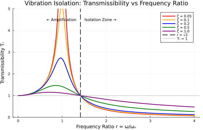
The key metric is transmissibility $T_r$—the ratio of transmitted force to applied force:

$$ T_r = \frac{F_T}{F_0} = \sqrt{ \frac{1 + (2\zeta r)^2}{(1 - r^2)^2 + (2\zeta r)^2} } $$

The $\sqrt{2}$ Rule

Why does $\sqrt{2}$ appear? At this frequency ratio, the numerator and denominator balance such that $T_r = 1$ regardless of damping. Below this point, the spring-mass system amplifies forces (you’re exciting near resonance). Above it, the mass’s inertia dominates—it “doesn’t want to move”—and transmitted forces drop.

Vibration Absorbers: Fighting Fire with Fire

What if a machine runs at a constant speed that coincides with its natural frequency? You can’t change the mass or speed—but you can add a Dynamic Vibration Absorber (DVA), also known as a Frahm damper or tuned mass damper.

How It Works

A DVA is a secondary mass-spring system $(m_2, k_2)$ attached to the main mass $(m_1, k_1)$. The magic happens when the absorber is tuned so that its natural frequency equals the forcing frequency:

$$ \omega_2 = \sqrt{\frac{k_2}{m_2}} = \omega \quad \text{(tuning condition)} $$

At this frequency, the absorber vibrates in such a way that it generates a force $k_2 X_2$ that exactly cancels the external excitation $F_0$. The main mass sits motionless while the absorber does all the work:

$$ X_1 = 0 \quad \text{and} \quad X_2 = -\frac{F_0}{k_2} $$

Mass Ratio Considerations

The mass ratio $\mu = m_2 / m_1$ affects how wide the effective frequency band is. A larger absorber mass gives a wider “notch” of suppression, but adds weight and cost. Typical values range from 5%–25% of the main mass.

Active Vibration Control

Traditional springs and dampers are passive—they react to forces with fixed characteristics. Modern high-performance systems use active vibration control with real-time feedback to achieve superior performance.

The Feedback Loop

An active system continuously measures the vibration state and applies a calculated counter-force:

1. Sensor measures displacement, velocity, or acceleration
2. Controller processes the signal and computes the required control force
3. Actuator applies the force to cancel or reduce vibration

Control Strategies

The most common approach is velocity feedback (skyhook damping), where the control force is proportional to velocity:

$$ F_c = -g \cdot \dot{x} \quad \text{(active damping)} $$

This effectively increases the damping coefficient without adding a physical damper. More sophisticated algorithms like LQR (Linear Quadratic Regulator) optimize the trade-off between vibration reduction and control effort.

Julia Example: Transmissibility Curve

Let’s visualize how transmissibility varies with frequency ratio for different damping values:

 1
 2
 3
 4
 5
 6
 7
 8
 9
10
11
12
13
14
15
16
17
18
19
20

using Plots

# Frequency ratio range
r = 0:0.01:4

# Damping ratios to compare
zeta_values = [0.05, 0.1, 0.2, 0.5, 1.0]

# Plot transmissibility for each damping ratio
p = plot(xlabel="r = ω/ωₙ", ylabel="Tᵣ", title="Transmissibility vs Frequency Ratio",
         ylims=(0, 5), legend=:topright, grid=true)

for ζ in zeta_values
    Tr = @. sqrt((1 + (2*ζ*r)^2) / ((1 - r^2)^2 + (2*ζ*r)^2))
    plot!(p, r, Tr, linewidth=2.5, label="ζ = $ζ")
end

# Mark crossover point
vline!(p, [sqrt(2)], linestyle=:dash, color=:black, label="r = √2")
hline!(p, [1], linestyle=:dot, color=:gray, label="Tᵣ = 1")

Expected Output:

1
2
3
4
5

Key Insights:
  • All curves cross at r = √2 ≈ 1.414
  • r < √2: Amplification (Tᵣ > 1)
  • r > √2: Isolation (Tᵣ < 1)
  • Higher ζ: better at resonance, worse at high frequencies

Summary

This post covered practical strategies for controlling mechanical vibrations:

What’s Next?

How do we actually measure vibration? The next post covers vibration measurement—sensors, signal processing, and machinery diagnostics.

References

Rao, S. S. (2018). Mechanical Vibrations (6th ed.). Pearson.