In our journey so far, we have lived in a world of “lumps.” We modeled cars, buildings, and machines as discrete masses connected by weightless springs and dampers. This is called a discrete system. Whether it had one degree of freedom or one hundred, the number was finite.

But look at a guitar string. Or a transmission shaft. Or an airplane wing. These aren’t just lumps of mass connected by springs; the mass and elasticity are distributed continuously throughout the material. These are Continuous Systems (or distributed systems).

Because every infinitesimal point on these bodies can move, they theoretically possess an infinite number of degrees of freedom. Consequently, they have an infinite number of natural frequencies.

In this post, based on Chapter 8 of Rao’s Mechanical Vibrations, we will explore the wave equations that govern strings, bars, and shafts, tackle the complex fourth-order differential equations of beams, and learn how to estimate frequencies using Rayleigh’s Method.

The Vibration of Strings: The Wave Equation

The simplest continuous system is a tightly stretched string—like a violin string or an overhead transmission cable.

Consider a string of length $l$ under tension $P$. If we take a tiny element of length $dx$ and apply Newton’s second law, we don’t get a standard differential equation; we get a Partial Differential Equation (PDE) because the deflection $w$ depends on both position $x$ and time $t$.

The Governing Equation

The equation of motion for free vibration is the classic Wave Equation:

$$\boxed{c^2 \frac{\partial^2 w}{\partial x^2} = \frac{\partial^2 w}{\partial t^2}}$$

The wave speed is determined by the tension-to-mass ratio:

$$ c = \sqrt{\frac{P}{\rho}} $$

Frequencies and Mode Shapes

For a string fixed at both ends (like a guitar string), the boundary conditions are $w(0,t)=0$ and $w(l,t)=0$. Solving the PDE reveals that the string can only vibrate at specific Natural Frequencies:

$$ \omega_n = \frac{n\pi c}{l} = \frac{n\pi}{l} \sqrt{\frac{P}{\rho}}, \quad n = 1, 2, 3, \dots $$

Associated with each frequency is a Mode Shape—a sine wave pattern:

$$ W_n(x) = \sin \left( \frac{n\pi x}{l} \right) $$

Bars and Shafts: Same Equation, Different Physics

The wave equation isn’t unique to strings. Longitudinal vibration of bars and torsional vibration of shafts follow identical mathematics—only the physical quantities differ.

Effect of Boundary Conditions

The same wave equation produces different frequency spectra depending on the boundary conditions:

Lateral Vibration of Beams: The Fourth-Order Challenge

The analysis complexity increases significantly when we move from axial to lateral (bending) vibration. Unlike strings that resist displacement through tension, beams resist through internal bending stiffness ($EI$).

The Euler-Bernoulli Beam Equation

The governing equation involves a fourth-order spatial derivative:

$$\boxed{\frac{\partial^2}{\partial x^2} \left[ EI \frac{\partial^2 w}{\partial x^2} \right] + \rho A \frac{\partial^2 w}{\partial t^2} = f(x,t)}$$

For a uniform beam in free vibration, this simplifies to:

$$ c^2 \frac{\partial^4 w}{\partial x^4} + \frac{\partial^2 w}{\partial t^2} = 0, \quad \text{where } c = \sqrt{\frac{EI}{\rho A}} $$

Why Four Boundary Conditions?

Since the equation is fourth-order in space, we need four boundary conditions (two at each end). This contrasts with strings and bars, which only need two.

Common Beam Configurations

Rayleigh’s Method: The Energy Shortcut

Solving PDEs analytically for complex structures—tapered wings, variable cross-sections, or unusual boundary conditions—is often intractable. Rayleigh’s Method provides an elegant alternative: estimate the fundamental frequency using energy principles without ever solving the differential equation.

The Core Idea: Energy Conservation

During free vibration, energy continuously transforms between two forms:

Conservation of energy demands:

$$\boxed{T_{max} = V_{max}}$$

The Recipe

1. Assume a mode shape $W(x)$ that satisfies the geometric boundary conditions
   • Good choices: static deflection curve, polynomial, or trigonometric function
2. Compute maximum kinetic energy: $T_{max} = \frac{1}{2}\omega^2 \int_0^L \rho A , W(x)^2 , dx$
3. Compute maximum potential energy: $V_{max} = \frac{1}{2} \int_0^L EI \left(\frac{d^2W}{dx^2}\right)^2 dx$ (for beams)
4. Equate and solve for $\omega$

Rayleigh’s Quotient

The result is a powerful formula that directly yields the frequency estimate:

$$ \omega^2 = \frac{\int_0^L EI \left(\dfrac{d^2W}{dx^2}\right)^2 dx}{\int_0^L \rho A , W(x)^2 , dx} = \frac{\text{Stiffness (curvature)}}{\text{Inertia (mass distribution)}} $$

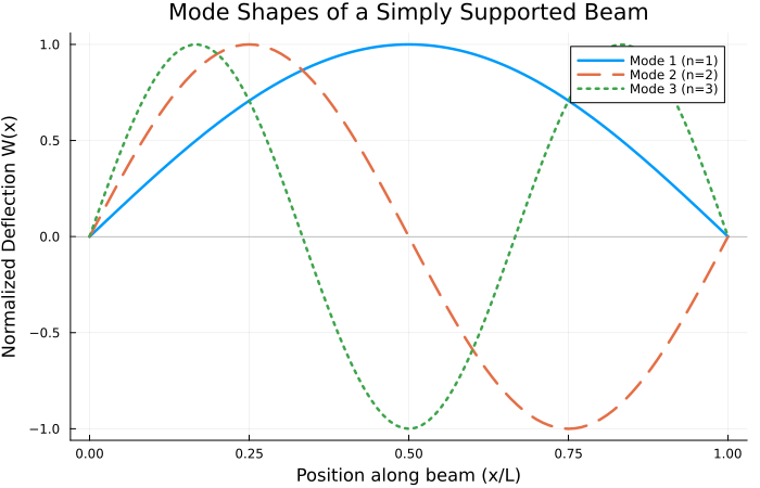
Julia Example: Plotting Beam Modes

Let’s visualize the first three mode shapes of a simply supported beam. The mode shapes are sinusoidal: $W_n(x) = \sin(n\pi x / L)$.

 1
 2
 3
 4
 5
 6
 7
 8
 9
10
11
12
13
14
15
16
17
18

using Plots

# Beam parameters
L = 1.0  # Length (normalized)
x = range(0, L, length=101)

# Mode shapes: Wₙ(x) = sin(nπx/L)
W1 = sin.(π .* x ./ L)      # Mode 1 (fundamental)
W2 = sin.(2π .* x ./ L)     # Mode 2
W3 = sin.(3π .* x ./ L)     # Mode 3

# Plot
plot(x, W1, linewidth=2.5, label="Mode 1 (n=1)")
plot!(x, W2, linewidth=2.5, linestyle=:dash, label="Mode 2 (n=2)")
plot!(x, W3, linewidth=2.5, linestyle=:dot, label="Mode 3 (n=3)")
xlabel!("Position along beam (x/L)")
ylabel!("Normalized Deflection W(x)")
title!("Mode Shapes of a Simply Supported Beam")

Expected Output:

1
2
3
4

Natural Frequency Ratios (relative to fundamental):
  Mode 1: ω1/ω₁ = 1
  Mode 2: ω2/ω₁ = 4
  Mode 3: ω3/ω₁ = 9

Summary

This post extended vibration analysis from discrete masses to continuous structures—systems with infinite degrees of freedom:

What’s Next?

How do we stop unwanted vibrations? The next post covers vibration control—isolation mounts, rotating machinery balancing, and dynamic vibration absorbers.

References

Rao, S. S. (2018). Mechanical Vibrations (6th ed.). Pearson.