MV-04: General Forcing Conditions – Fourier, Convolution, and Response Spectra
So far, we have analyzed systems subjected to smooth, repeating harmonic forces—like the rotation of a motor or the vibration of an unbalanced wheel. But the real world is rarely so predictable.
What happens when a car hits a pothole? How does a building respond to the chaotic shaking of an earthquake? What about the sudden blast pressure on a protective structure? These are not harmonic forces—they are irregular, transient, and sometimes violent.
This post, based on Chapter 4 of Rao’s Mechanical Vibrations, explores how engineers analyze systems under General Forcing Conditions. We will move from the frequency domain (Fourier Series) to the time domain (Convolution Integral), and introduce the practical design tool: the Response Spectrum.
Periodic but Non-Harmonic: The Power of Fourier Series
Not all repeating forces are smooth sine waves. Consider the force exerted by a cam mechanism or the pressure fluctuations in a reciprocating compressor. These are periodic (they repeat after a time interval $\tau$), but they are non-harmonic.
The solution comes from the French mathematician Jean Baptiste Joseph Fourier: Any periodic function, no matter how complex, can be represented as a sum of simple harmonic functions.
$$ F(t) = \frac{a_0}{2} + \sum_{j=1}^{\infty} \left[ a_j \cos(j\omega t) + b_j \sin(j\omega t) \right] $$
where the coefficients $a_j$ and $b_j$ are determined by integration over one period.

The Superposition Principle
Because linear vibration systems obey superposition, we can:
- Decompose the complex force into individual harmonics
- Solve for the response to each harmonic separately (using methods from the previous post)
- Sum all individual responses to obtain the total system response
Non-Periodic Forces: The Convolution Integral
What if the force doesn’t repeat? Consider a hammer striking an anvil, a package dropped on the floor, or the ground motion during an earthquake. These are transient excitations that cannot be handled by Fourier methods.
The Impulse Response Function
The key insight is the unit impulse $\delta(t)$—a force of infinite magnitude acting for an infinitesimal duration, with unit area. When a system is struck by a unit impulse, its response is the Impulse Response Function $g(t)$:
$$ g(t) = \frac{e^{-\zeta \omega_n t}}{m \omega_d} \sin(\omega_d t), \quad t \geq 0 $$
This describes how the system “rings” after being struck—like a bell after a single tap.
The Convolution (Duhamel) Integral
The genius of this approach: treat any arbitrary force $F(t)$ as a series of infinitesimal impulses. Each impulse at time $\tau$ contributes to the response at time $t$. Summing all contributions gives the Convolution Integral:
$$ x(t) = \int_0^t F(\tau) , g(t - \tau) , d\tau $$

Earthquake Engineering: The Response Spectrum
Computing the exact time history for a building during an earthquake is computationally expensive, and every earthquake is unique. For design purposes, engineers care primarily about the maximum response—peak displacement or acceleration—rather than the precise motion at every instant.
This leads to the Response Spectrum, a fundamental tool in seismic design.
What is a Response Spectrum?
A response spectrum plots the maximum response of SDOF systems against their natural period $T$ for a specific ground motion record. The construction process:
- Apply an earthquake record to a SDOF system with period $T_1$, record maximum response
- Repeat for systems with periods $T_2, T_3, \ldots, T_n$
- Plot all maximum values to create the spectrum

Types of Response Spectra
| Type | Symbol | Description |
|---|---|---|
| Displacement | $S_d$ | Maximum relative displacement |
| Velocity | $S_v$ | Maximum relative velocity (≈ $\omega_n S_d$) |
| Acceleration | $S_a$ | Maximum absolute acceleration (≈ $\omega_n^2 S_d$) |
Laplace Transforms: Handling Discontinuities
When forcing functions are discontinuous—like a step force (suddenly applying a load) or a ramp force (linearly increasing load)—the Laplace Transform provides an efficient analytical solution.
The Laplace transform $\mathcal{L}{f(t)} = F(s) = \int_0^\infty f(t)e^{-st}dt$ converts time-domain differential equations into algebraic equations in the complex $s$-domain.
Why it works: Derivatives become multiplications by $s$:
- $\mathcal{L}{\dot{x}} = sX(s) - x(0)$
- $\mathcal{L}{\ddot{x}} = s^2X(s) - sx(0) - \dot{x}(0)$
This transforms our equation of motion $m\ddot{x} + c\dot{x} + kx = F(t)$ into:
$$ X(s) = \frac{F(s) + \text{(initial conditions)}}{ms^2 + cs + k} $$
The solution is then obtained by inverse Laplace transform, often using partial fractions and standard transform tables.
Key Observations
| Input Type | Peak Response | Characteristic |
|---|---|---|
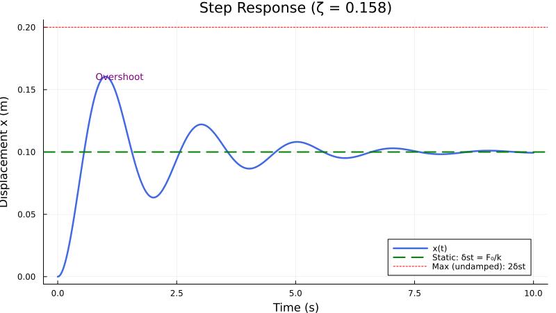
| Step | $2\delta_{st}$ (undamped) | Sudden application causes overshoot |
| Ramp | ≈ $\delta_{st}$ | Gradual increase minimizes overshoot |

Julia Example: Response to a Step Force
Let’s visualize the response of an underdamped system to a step force (sudden constant load). As noted above, we expect the system to overshoot the static equilibrium position before settling.
| |
Summary
This post moved beyond harmonic excitation into the realm of general forcing conditions:
| Method | Application | Key Feature |
|---|---|---|
| Fourier Series | Periodic non-harmonic forces | Decomposes into harmonics |
| Convolution Integral | Arbitrary transient forces | Uses impulse response function |
| Response Spectrum | Earthquake design | Maximum response vs period |
| Laplace Transform | Step/ramp/discontinuous forces | Converts to algebraic equations |
What’s Next?
So far, we have analyzed single-mass systems. But most real machines have multiple moving parts. In the next post, we will explore Two-Degree-of-Freedom Systems—what happens when two masses interact and exchange energy.
References
Rao, S. S. (2018). Mechanical Vibrations (6th ed.). Pearson.