So far, we have learned how to model systems and observed how they vibrate freely under initial disturbances. But in the real world, systems rarely exist in isolation—they are pushed, pulled, and shaken by the environment around them.

When an external force follows a repeating pattern—like the hum of an electric motor, the rotation of a turbine, or the shake of a washing machine—we call it Harmonically Excited Vibration. This is perhaps the most important topic in vibration analysis because it introduces the engineer’s greatest challenge: Resonance.

In this post, based on Chapter 3 of Rao’s Mechanical Vibrations, we will explore how systems respond to rhythmic forces, why rotating machines shake, and how to isolate sensitive equipment from a vibrating environment.

The Equation of Motion: Steady-State vs. Transient

Consider our standard spring-mass-damper system, now subjected to a continuous harmonic force $F(t) = F_0 \cos(\omega t)$. The equation of motion becomes:

$$ m\ddot{x} + c\dot{x} + kx = F_0 \cos(\omega t) $$

The complete solution to this differential equation consists of two distinct parts:

1. Transient Response ($x_h$): The homogeneous solution representing free vibration. Due to damping, this component decays exponentially and eventually vanishes.
2. Steady-State Response ($x_p$): The particular solution representing the motion driven by the external force. This persists as long as the force is applied.

In forced vibration analysis, engineers focus primarily on the steady-state response—the long-term behavior after initial transients have died out.

The Undamped System: Resonance and Beating

To understand the fundamental physics, consider an undamped system ($c=0$). The response amplitude depends critically on the Frequency Ratio $r = \omega / \omega_n$—the relationship between the forcing frequency and the system’s natural frequency.

For an undamped system, the magnification factor is: $$ M = \frac{X}{\delta_{st}} = \frac{1}{|1 - r^2|} $$

where $\delta_{st} = F_0/k$ is the static deflection under the force amplitude.

The Danger Zone: Resonance

When $r = 1$ (forcing frequency equals natural frequency), the denominator vanishes and amplitude theoretically grows to infinity. This catastrophic condition is called Resonance.

The Beating Phenomenon

When the forcing frequency is close to but not equal to the natural frequency ($\omega \approx \omega_n$), a fascinating phenomenon called Beating occurs. The amplitude oscillates in a rhythmic pulsation as the free and forced vibrations alternately reinforce and cancel each other.

The beat frequency is $\omega_{beat} = |\omega - \omega_n|$, which is audible as the distinctive “waa-waa-waa” sound when twin aircraft engines are slightly out of sync.

Adding Damping: The Reality Check

In real systems, damping prevents the amplitude from reaching infinity at resonance. For a viscously damped system, the magnification factor becomes:

$$ M = \frac{X}{\delta_{st}} = \frac{1}{\sqrt{(1 - r^2)^2 + (2\zeta r)^2}} $$

The effect of damping ratio $\zeta$ on the frequency response is profound:

• Low damping (ζ < 0.1): Sharp resonance peak, sensitive to frequency
• Moderate damping (0.1 < ζ < 0.5): Reduced peak, broader response
• High damping (ζ > 0.7): Nearly flat response, no distinct peak

The phase relationship (discussed earlier) remains important: the response always lags the force by 90° at the resonance frequency, regardless of damping level.

Practical Application: Rotating Unbalance

Rotating unbalance is one of the most common vibration sources in mechanical engineering. When a rotating component (motor rotor, washing machine drum, turbine) has uneven mass distribution, the eccentric mass generates a centrifugal force that excites vibration.

For an eccentric mass $m$ at radius $e$ rotating at angular velocity $\omega$, the excitation force is $F = me\omega^2$. The equation of motion becomes:

$$ M\ddot{x} + c\dot{x} + kx = me\omega^2 \sin(\omega t) $$

The dimensionless amplitude response is: $$ \frac{MX}{me} = \frac{r^2}{\sqrt{(1-r^2)^2 + (2\zeta r)^2}} $$

Practical Application: Base Excitation and Isolation

When vibration comes from the ground rather than the machine—like a car on a bumpy road or equipment near heavy machinery—we call this Base Excitation. The key metric is Displacement Transmissibility $T_d$, which measures how much ground motion gets transmitted to the mass:

$$ T_d = \frac{X}{Y} = \sqrt{ \frac{1 + (2\zeta r)^2}{(1-r^2)^2 + (2\zeta r)^2} }$$

The Critical Design Rule

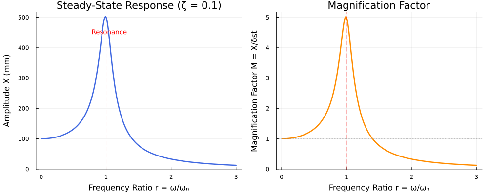
Julia in Action: Frequency Response

Engineers often use frequency response plots to visualize how a system responds across a range of frequencies. The following Julia code calculates and plots the steady-state response amplitude for a damped system.

 1
 2
 3
 4
 5
 6
 7
 8
 9
10
11
12
13
14
15
16
17
18
19
20
21
22
23
24
25
26
27
28
29
30

using Plots

# System Parameters
m = 10.0        # Mass (kg)
k = 1000.0      # Stiffness (N/m)
c = 20.0        # Damping (N·s/m)
F0 = 100.0      # Force Amplitude (N)

# Derived Parameters
ωn = sqrt(k/m)              # Natural Frequency (rad/s)
ζ = c / (2*sqrt(k*m))       # Damping Ratio

# Frequency Range (0 to 3 times natural frequency)
ω = range(0.1, 3*ωn, length=300)
r = ω ./ ωn                 # Frequency Ratio

# Steady-State Amplitude
X = @. F0 / sqrt((k - m*ω^2)^2 + (c*ω)^2)

# Plot
plot(r, X .* 1000,  # Convert to mm
    linewidth = 2.5,
    xlabel = "Frequency Ratio r = ω/ωₙ",
    ylabel = "Amplitude X (mm)",
    title = "Steady-State Response (ζ = $(round(ζ, digits=3)))",
    legend = false, grid = true
)
vline!([1.0], linestyle=:dash, color=:red, label="Resonance")

savefig("frequency_response.png")

Summary

In this post, we’ve moved from free vibration to the rhythmic world of forced vibration. We’ve seen that:

1. Resonance occurs when the forcing frequency matches the natural frequency, leading to maximum amplitude.
2. Damping is the primary factor limiting vibration amplitude at resonance.
3. Isolation (protecting a mass from base motion) requires a frequency ratio $r > \sqrt{2}$.

What’s Next?

Life isn’t always a smooth sine wave. In the next post, “Vibration Under General Forcing Conditions,” we will learn how to handle shock loadings, pulses, and irregular forces using the Fourier Series and Convolution Integral.

References

Rao, S. S. (2018). Mechanical Vibrations (6th ed.). Pearson.