Metal Fracture Simulation: Comparing Morse and EAM Potentials in LAMMPS

Publish on: 2022/06/08 Classify at: RESEARCH/Simulation

Words: 1961 Read:≈ 10min

Summary

A hands-on tutorial on simulating tensile fracture in copper using LAMMPS. We compare the simplified Morse potential with the accurate EAM potential and analyze stress-strain behavior during crack propagation.

Understanding how materials fail is fundamental to engineering. Molecular Dynamics (MD) allows us to peek into the atomic scale and observe the precise mechanisms of fracture—something impossible in typical experiments.

In this tutorial, we will verify the behavior of Mode I tensile fracture in a Copper single crystal using LAMMPS. We’ll compare a quick-and-dirty Morse potential against a research-grade EAM potential to see why the choice of physics model matters.

Simulation Preview: Atomic-scale view of Mode I crack propagation in Copper.

In this post, we will:

Derive the Physics: Understand stress, strain, and atomic potentials.
Compare Models: Contrast the simple Morse potential with the accurate Embedded Atom Method (EAM).
Code in LAMMPS: Build complete simulation scripts from scratch.
Analyze Results: Visualize crack propagation and interpret stress-strain curves.

The Physics: Fracture Mechanics at Atomic Scale

Stress and Strain

When a material is pulled, it stretches. At the atomic level, this stretches the bonds between atoms.

$$ \sigma = E \cdot \varepsilon \quad \text{(Elastic Region)} $$

Where:

$\sigma$: Engineering stress (force per unit area)
$E$: Young’s modulus (material stiffness)
$\varepsilon$: Engineering strain (change in length / original length)

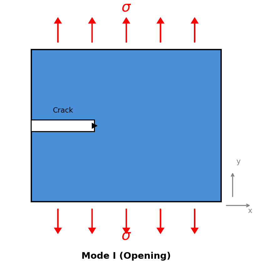
Mode I Fracture

Mode I (Opening Mode) is the most common failure type, where tensile stress pulls the crack faces directly apart. It’s the “tearing” mode of fracture.

Mode I (Opening) Fracture: Tensile stress applied perpendicular to the crack.

At the atomic scale, fracture isn’t just a clean break. It involves:

Bond Stretching: Atoms at the crack tip differ from the bulk.
Bond Breaking: When local stress exceeds bond strength.
Dissipation: Energy loss through heat or plastic deformation (dislocation movement).

Interatomic Potentials: Morse vs EAM

The “brain” of any MD simulation is the interatomic potential—the mathematical rule describing how atoms interact. We’ll compare two vastly different approaches:

Why the Choice Matters

Pair Potentials (e.g., Morse): Assume interaction depends only on the distance between two atoms. Simple, but ignores the “electron glue” effect in metals.
Many-Body Potentials (e.g., EAM): Account for the local electron density. An atom “feels” difference based on how many neighbors it has. This is critical for surfaces and cracks.

Morse Potential (Simplified)

The Morse potential is a computationally cheap pair potential:

$$ V(r) = D_0 \left[ e^{-2\alpha(r-r_0)} - 2e^{-\alpha(r-r_0)} \right] $$

Where:

$D_0$: Bond dissociation energy (0.3429 eV for Cu)
$\alpha$: Controls potential width (1.3588 Å⁻¹)
$r_0$: Equilibrium bond distance (2.866 Å)

Pros: Simple, fast, no external files needed
Cons: Poor description of metallic bonding, inaccurate surface energies

EAM Potential (Accurate)

The Embedded Atom Method (EAM) captures the many-body nature of metallic bonding:

$$ E_i = F_i(\bar{\rho}_i) + \frac{1}{2} \sum_{j \neq i} \phi_{ij}(r_{ij}) $$

Where:

$F_i$: Embedding energy (energy to place atom in electron density $\bar{\rho}$)
$\bar{\rho}_i$: Background electron density at atom $i$
$\phi_{ij}$: Pair interaction between atoms $i$ and $j$

Pros: Accurate surface energies, stacking fault energies, and elastic constants
Cons: Requires external potential file, computationally more expensive

Simulation Setup

Both simulations use identical loading conditions for fair comparison:

Parameter	Morse (Simple)	EAM (Full)
Material	Cu (FCC)	Cu (FCC)
Lattice constant	3.615 Å	3.615 Å
Atoms	~1,000	~8,000
Box size	16×8×2 lattice	28×14×4 lattice
Crack length	~1/3 width	~1/3 width
Temperature	300 K	300 K
Pull velocity	0.5 Å/ps	0.5 Å/ps
Timestep	1 fs	1 fs
Simulation time	50 ps	50 ps

LAMMPS Implementation

We will build two versions of the simulation:

Standalone Version: Uses the Morse potential. No external download required. Good for testing.
Production Version: Uses the EAM potential. Requires a specific potential file. Good for physics.

Morse Potential Version (Standalone)

This script is self-contained. You can copy-paste and run it immediately.

  1
  2
  3
  4
  5
  6
  7
  8
  9
 10
 11
 12
 13
 14
 15
 16
 17
 18
 19
 20
 21
 22
 23
 24
 25
 26
 27
 28
 29
 30
 31
 32
 33
 34
 35
 36
 37
 38
 39
 40
 41
 42
 43
 44
 45
 46
 47
 48
 49
 50
 51
 52
 53
 54
 55
 56
 57
 58
 59
 60
 61
 62
 63
 64
 65
 66
 67
 68
 69
 70
 71
 72
 73
 74
 75
 76
 77
 78
 79
 80
 81
 82
 83
 84
 85
 86
 87
 88
 89
 90
 91
 92
 93
 94
 95
 96
 97
 98
 99
100
101
102
103
104
105
106
107
108
109
110
111
112
113
114
115
116
117
118
119
120
121
122
123
124
125
126
127
128
129
130
131
132
133
# ==============================================================================
# Metal Fracture Simulation - Simplified Version (No External Potential File)
# ==============================================================================
# Uses Morse potential as an approximation for copper.
# This version can run without downloading external EAM files.
#
# Author: MD Tutorial
# Units: Metal units (Angstroms, eV, ps, K)
# ==============================================================================

# Create output directory
shell           mkdir -p fracture_results_morse

# =====================
# 1. Initialization
# =====================
units           metal
dimension       3
boundary        p s p          # Periodic in x,z; free surface in y
atom_style      atomic

# =====================
# 2. Create Copper Crystal (FCC)
# =====================
lattice         fcc 3.615 orient x 1 0 0 orient y 0 1 0 orient z 0 0 1

# Smaller box for faster testing: ~60 x 30 x 7 Angstroms (~3000 atoms)
region          box block 0 16 0 8 0 2 units lattice
create_box      1 box
create_atoms    1 box

# =====================
# 3. Create Pre-existing Crack
# =====================
region          crack block 0 5 3.5 4.5 INF INF units lattice
delete_atoms    region crack

variable        natoms equal count(all)
print           "Atoms after crack: ${natoms}"

# =====================
# 4. Morse Potential (Approximation for Cu)
# =====================
# Morse parameters fitted to Cu properties
# D0 = 0.3429 eV, alpha = 1.3588 /Angstrom, r0 = 2.866 Angstrom
pair_style      morse 6.0
pair_coeff      1 1 0.3429 1.3588 2.866
mass            1 63.546  # Cu atomic mass

# =====================
# 5. Define Regions and Groups
# =====================
region          top_grip block INF INF 7 INF INF INF units lattice
region          bot_grip block INF INF INF 1 INF INF units lattice

group           top_atoms region top_grip
group           bot_atoms region bot_grip
group           boundary union top_atoms bot_atoms
group           mobile subtract all boundary

# =====================
# 6. Minimize Initial Structure
# =====================
minimize        1.0e-4 1.0e-6 500 5000

# =====================
# 7. Initialize Temperature
# =====================
velocity        mobile create 300.0 54321 mom yes rot yes

# =====================
# 8. Compute Properties
# =====================
compute         csym all centro/atom fcc
compute         pe all pe/atom
compute         ke all ke/atom

# Compute stress tensor for pressure components
compute         stress all pressure thermo_temp

# =====================
# 9. Equilibration
# =====================
fix             eq mobile nvt temp 300.0 300.0 0.1
timestep        0.001

thermo          200
thermo_style    custom step temp pe ke etotal press c_stress[2]

run             1000
unfix           eq

# =====================
# 10. Apply Tensile Loading
# =====================
# Pull velocity: 0.5 Angstrom/ps (10x faster for visible fracture)
variable        pull_vel equal 0.5

# Store initial box length for strain calculation
variable        Ly0 equal ly

# Fix bottom atoms completely
fix             fix_bot bot_atoms setforce 0.0 0.0 0.0
velocity        bot_atoms set 0.0 0.0 0.0

# Apply constant velocity to top atoms (pull upward)
fix             pull_top top_atoms move linear 0.0 ${pull_vel} 0.0 units box

fix             nve mobile nve

# Track strain and stress
variable        strain equal (step-1007)*dt*v_pull_vel/v_Ly0
variable        stress equal -c_stress[2]/10000  # GPa (pyy component)

# =====================
# 11. Output
# =====================
thermo          500
thermo_style    custom step temp v_strain v_stress pe etotal

# Trajectory for OVITO visualization
dump            viz all custom 200 fracture_results_morse/fracture.*.dump id type x y z c_csym c_pe

# Stress-strain curve
fix             ss_out all print 100 "${strain} ${stress}" &
                file fracture_results_morse/stress_strain_morse.dat screen no title "strain stress_GPa"

# =====================
# 12. Run Fracture Simulation
# =====================
run             50000

print           "=== Simulation Complete ==="

EAM Potential Version (Production)

For physically accurate results, we switch to the EAM potential. The logic is identical, except for the pair_style and box size.

 1
 2
 3
 4
 5
 6
 7
 8
 9
10
11
12
13
14
15
16
17
18
19
20
21
22
23
24
25
26
27
28
29
30
31
32
33
34
35
36
37
38
39
40
41
42
43
44
45
46
47
48
49
50
51
52
53
54
55
56
57
58
59
60
61
62
63
64
65
# ==============================================================================
# Metal Fracture Simulation - Full Version (EAM Potential)
# ==============================================================================
# Uses EAM potential for accurate copper properties.
# Requires: Cu_mishin1.eam.alloy (download from NIST potentials repository)
#
# Author: MD Tutorial
# Units: Metal units (Angstroms, eV, ps, K)
# ==============================================================================

# Create output directory
shell           mkdir -p fracture_results_eam

# =====================
# 1. Initialization
# =====================
units           metal
dimension       3
boundary        p s p          # Periodic in x,z; free surface in y
atom_style      atomic

# =====================
# 2. Create Copper Crystal (FCC)
# =====================
lattice         fcc 3.615 orient x 1 0 0 orient y 0 1 0 orient z 0 0 1

# Larger box: ~100 x 50 x 14 Angstroms (~8000 atoms)
region          box block 0 28 0 14 0 4 units lattice
create_box      1 box
create_atoms    1 box

# =====================
# 3. Create Pre-existing Crack
# =====================
region          crack block 0 9 6.5 7.5 INF INF units lattice
delete_atoms    region crack

variable        natoms equal count(all)
print           "Atoms after crack: ${natoms}"

# =====================
# 4. EAM Potential for Copper
# =====================
# Mishin EAM potential - accurate for Cu mechanical properties
# Download from: https://www.ctcms.nist.gov/potentials/
pair_style      eam/alloy
pair_coeff      * * Cu_mishin1.eam.alloy Cu

# =====================
# 5. Define Regions and Groups
# =====================
region          top_grip block INF INF 13 INF INF INF units lattice
region          bot_grip block INF INF INF 1 INF INF units lattice

group           top_atoms region top_grip
group           bot_atoms region bot_grip
group           boundary union top_atoms bot_atoms
group           mobile subtract all boundary

# =====================
# 6-12. Same as Morse version...
# =====================
# (See full script in repository)

run             50000

Download EAM Potential File:

`1`	`wget https://www.ctcms.nist.gov/potentials/entry/2001--Mishin-Y-Mehl-M-J-Papaconstantopoulos-D-A-et-al--Cu-1/`

Running the Simulations

Execute both simulations:

1
2
3
4
5
# Run simplified version (no dependencies)
lmp -in metal_fracture_simple.in

# Run full version (requires EAM file)
lmp -in metal_fracture.in

Results and Analysis

Stress-Strain Curves

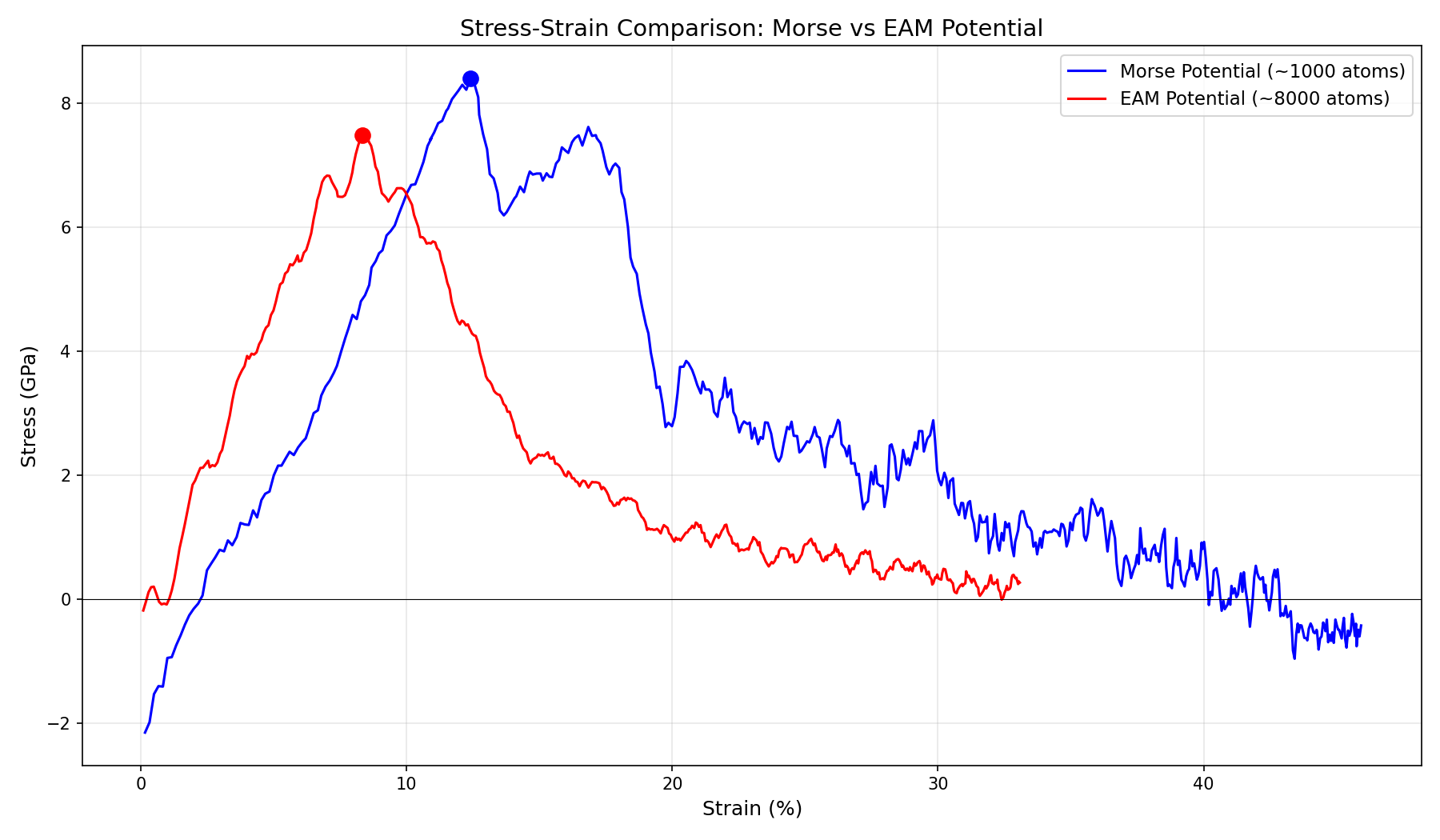
Stress-Strain Comparison: Morse vs EAM Potential

The stress-strain curves reveal distinct mechanical behaviors:

Property	Morse Potential	EAM Potential
Peak Stress	~8.4 GPa	~7.5 GPa
Strain at Peak	~12%	~8%
Post-Peak Behavior	Gradual decline	Sharp drop
Failure Mode	Ductile-like	Brittle-like

Visualizing Crack Propagation

Since the stress-strain curves suggest different failure modes, let’s look at the atomic trajectories.

Key Observations

Peak Strength: Both predict ~7-8 GPa. This is theoretically reasonable for a flawed crystal at these high strain rates, but much higher than bulk experimental copper.
Failure Strain: Morse stretches to ~12% strain, behaving like “gum”. EAM snaps at ~8%, capturing the brittle nature of high-speed fracture.
Mechanism: EAM accurately captures the surface energy cost of creating a new crack surface. Morse underestimates this, allowing the material to resist fracture longer.
Snap-back: The sharp drop in the EAM curve (Brittle) vs the gradual decline in Morse (Ductile) is the signature difference.

Summary and Recommendations

When to Use Each Potential

Use Case	Recommended Potential
Learning/Testing	Morse
Quick prototyping	Morse
Qualitative trends	Morse
Publication-quality	EAM
Quantitative predictions	EAM
Multi-element systems	EAM/MEAM

Key Takeaways

Potentials are Physics: They aren’t just parameters. Morse gives you “balls on springs”. EAM gives you “atoms in an electron sea”.
Surface Energy Drives Fracture: Creating a crack means creating surface. If your potential gets surface energy wrong (like Morse), your fracture mechanics will be wrong.
Timescales Matter: MD happens in picoseconds. The strain rates ($10^9 s^{-1}$) are explosive. Don’t expect to match macroscopic tensile test numbers directly.

References

Mishin, Y., et al. “Structural stability and lattice defects in copper: Ab initio, tight-binding, and embedded-atom calculations.” Physical Review B 63.22 (2001): 224106.
Farkas, D. “Atomistic simulations of metallic microstructures.” Current Opinion in Solid State and Materials Science 17.6 (2013): 284-297.
LAMMPS Documentation: https://docs.lammps.org/
NIST Interatomic Potentials Repository: https://www.ctcms.nist.gov/potentials/