Molecular Dynamics 101: From First Principles to Python, Julia, and LAMMPS

Publish on: 2022/06/05 Classify at: RESEARCH/Simulation

Words: 2134 Read:≈ 11min

Summary

A deep dive into the 'Hello World' of Molecular Dynamics: simulating Lennard-Jones Argon. We derive the physics, build a scratch implementation in Python and Julia, and compare it with production-grade LAMMPS scripts.

Molecular Dynamics (MD) simulation is a powerful computational window into the microscopic world. By numerically solving Newton’s equations of motion ($F=ma$) for a system of interacting particles, we can predict macroscopic properties—like temperature, pressure, and diffusion coefficients—from first principles.

For beginners and algorithm validation, the Lennard-Jones (L-J) fluid (typically modeling Liquid Argon) is the classic “Hello World” case. It covers all the core elements of MD: identifying interaction potentials, applying boundary conditions, and integrating equations of motion.

In this post, we will:

Derive the physics behind the L-J potential and force calculations
Implement the simulation from scratch in both Python and Julia
Compare our results with production-grade LAMMPS simulations
Benchmark performance across all three approaches

The Physics: Lennard-Jones Potential

Before writing any code, we need to understand the physics. In classical MD, the most critical input is the potential energy surface—a function describing how atoms interact. For noble gases like Argon, the Lennard-Jones 12-6 potential is the standard model:

$$ V(r) = 4\epsilon \left[ \left( \frac{\sigma}{r} \right)^{12} - \left( \frac{\sigma}{r} \right)^6 \right] $$

Where:

$V(r)$: Potential energy at distance $r$.
$\epsilon$ (epsilon): Depth of the potential well (strength of attraction).
$\sigma$ (sigma): Finite distance where the inter-particle potential is zero.
$r^{-12}$ term: Short-range repulsion (Pauli exclusion principle).
$r^{-6}$ term: Long-range attraction (Van der Waals/dispersion forces).

Force Calculation

To move atoms, we need forces. The force is the negative gradient of the potential:

$$ \vec{F} = -\nabla V(r) $$

Analytically derived from the L-J potential:

$$ \vec{F}(r) = \frac{24\epsilon}{r^2} \left[ 2\left( \frac{\sigma}{r} \right)^{12} - \left( \frac{\sigma}{r} \right)^6 \right] \vec{r} $$

Core Algorithm Logic

With the physics in hand, let’s outline the computational workflow. A working MD simulation must address four key challenges:

Initialization: Place atoms in a box (usually avoiding overlap) and assign initial velocities based on the Maxwell-Boltzmann distribution for the target temperature.
Periodic Boundary Conditions (PBC): To simulate an infinite bulk fluid using a small box, particles leaving one side re-enter from the opposite side.
Minimum Image Convention: When calculating forces, a particle interacts with the closest image of its neighbor (whether in the primary box or a periodic replica).
Integration (Velocity Verlet): A symplectic integrator that preserves energy well over long times.

Velocity Verlet Steps:

Update position: $ \vec{r}(t+\Delta t) = \vec{r}(t) + \vec{v}(t)\Delta t + \frac{1}{2}\vec{a}(t)\Delta t^2 $
Calculate new forces and acceleration: $\vec{a}(t+\Delta t)$
Update velocity: $ \vec{v}(t+\Delta t) = \vec{v}(t) + \frac{1}{2}[\vec{a}(t) + \vec{a}(t+\Delta t)]\Delta t $

Simulation Parameters

Now let’s get concrete. To ensure a fair comparison, all three implementations use identical parameters:

Parameter	Value	Description
N (particles)	64	Number of atoms
L (box size)	10.0 σ	Simulation box dimension
ρ (density)	0.64	N/L² in reduced units
dt (timestep)	0.01 τ	Integration time step
T (temperature)	1.0 ε/kB	Target temperature
rc (cutoff)	3.0 σ	L-J potential cutoff
Steps	1000	Total simulation steps
Ensemble	NVE	Microcanonical

Python Implementation (From Scratch)

Let’s start with Python—the best choice for understanding the algorithm. This implementation prioritizes readability over speed, using NumPy for vector operations while avoiding complex optimizations like neighbor lists.

  1
  2
  3
  4
  5
  6
  7
  8
  9
 10
 11
 12
 13
 14
 15
 16
 17
 18
 19
 20
 21
 22
 23
 24
 25
 26
 27
 28
 29
 30
 31
 32
 33
 34
 35
 36
 37
 38
 39
 40
 41
 42
 43
 44
 45
 46
 47
 48
 49
 50
 51
 52
 53
 54
 55
 56
 57
 58
 59
 60
 61
 62
 63
 64
 65
 66
 67
 68
 69
 70
 71
 72
 73
 74
 75
 76
 77
 78
 79
 80
 81
 82
 83
 84
 85
 86
 87
 88
 89
 90
 91
 92
 93
 94
 95
 96
 97
 98
 99
100
101
102
103
104
105
106
107
108
109
110
111
112
113
"""
Lennard-Jones Molecular Dynamics Simulation in Python
Units: Reduced Lennard-Jones units (epsilon=1, sigma=1, mass=1)
"""

import numpy as np
import time
import json
import os


class MDSimulation:
    """
    Molecular Dynamics simulation class for a 2D Lennard-Jones fluid.
    """
    
    def __init__(self, n_particles: int, box_size: float, n_steps: int, dt: float, temp: float):
        """Initialize the MD simulation with given parameters."""
        self.N = n_particles
        self.L = box_size
        self.dt = dt
        self.n_steps = n_steps
        self.target_temp = temp
        self.cutoff_sq = 9.0  # 3.0^2
        
        # Initialize positions on a grid
        self._initialize_positions()
        self._initialize_velocities()
        self.acc = np.zeros((self.N, 2), dtype=np.float64)
        self.energies = []
        
    def _initialize_positions(self):
        """Place particles on a regular grid to avoid initial overlaps."""
        n_dim = int(np.ceil(np.sqrt(self.N)))
        spacing = self.L / n_dim
        indices = np.arange(self.N)
        self.pos = np.zeros((self.N, 2), dtype=np.float64)
        self.pos[:, 0] = (indices % n_dim + 0.5) * spacing
        self.pos[:, 1] = (indices // n_dim + 0.5) * spacing
        
    def _initialize_velocities(self):
        """Initialize velocities from Maxwell-Boltzmann distribution."""
        self.vel = np.random.randn(self.N, 2).astype(np.float64)
        self.vel -= np.mean(self.vel, axis=0)  # Remove COM velocity
        current_temp = np.sum(self.vel ** 2) / (2 * self.N)
        if current_temp > 0:
            self.vel *= np.sqrt(self.target_temp / current_temp)
    
    def compute_forces(self) -> float:
        """
        Compute pairwise Lennard-Jones forces using minimum image convention.
        Returns total potential energy.
        """
        potential_energy = 0.0
        self.acc.fill(0.0)
        
        for i in range(self.N):
            for j in range(i + 1, self.N):
                dr = self.pos[i] - self.pos[j]
                dr -= self.L * np.round(dr / self.L)  # Minimum image
                r2 = np.dot(dr, dr)
                
                if r2 < self.cutoff_sq:
                    r2_inv = 1.0 / r2
                    r6_inv = r2_inv ** 3
                    r12_inv = r6_inv ** 2
                    
                    f_scalar = 24.0 * (2.0 * r12_inv - r6_inv) * r2_inv
                    f_vec = f_scalar * dr
                    
                    self.acc[i] += f_vec
                    self.acc[j] -= f_vec
                    potential_energy += 4.0 * (r12_inv - r6_inv)
        
        return potential_energy
    
    def integrate(self) -> tuple:
        """Perform one step of Velocity Verlet integration."""
        dt, dt_sq_half = self.dt, 0.5 * self.dt * self.dt
        
        self.pos += self.vel * dt + self.acc * dt_sq_half
        self.pos = np.mod(self.pos, self.L)  # PBC
        
        acc_old = self.acc.copy()
        pot_eng = self.compute_forces()
        self.vel += 0.5 * (acc_old + self.acc) * dt
        kin_eng = 0.5 * np.sum(self.vel ** 2)
        
        return pot_eng, kin_eng
    
    def run(self, verbose: bool = True) -> dict:
        """Run the MD simulation."""
        self.compute_forces()
        start_time = time.perf_counter()
        
        for step in range(self.n_steps):
            pe, ke = self.integrate()
            self.energies.append([pe, ke, pe + ke])
        
        elapsed = time.perf_counter() - start_time
        return {
            "elapsed_time": elapsed,
            "steps_per_second": self.n_steps / elapsed,
            "energies": np.array(self.energies)
        }


if __name__ == "__main__":
    np.random.seed(42)
    sim = MDSimulation(64, 10.0, 1000, 0.01, 1.0)
    results = sim.run()
    print(f"Completed in {results['elapsed_time']:.4f}s")
    print(f"Performance: {results['steps_per_second']:.2f} steps/sec")

Julia Implementation (High Performance)

Python is excellent for prototyping, but those nested for loops are painfully slow. Enter Julia—a language that combines Python’s readability with C-level performance. The algorithm is identical; the difference is that Julia compiles to efficient machine code.

  1
  2
  3
  4
  5
  6
  7
  8
  9
 10
 11
 12
 13
 14
 15
 16
 17
 18
 19
 20
 21
 22
 23
 24
 25
 26
 27
 28
 29
 30
 31
 32
 33
 34
 35
 36
 37
 38
 39
 40
 41
 42
 43
 44
 45
 46
 47
 48
 49
 50
 51
 52
 53
 54
 55
 56
 57
 58
 59
 60
 61
 62
 63
 64
 65
 66
 67
 68
 69
 70
 71
 72
 73
 74
 75
 76
 77
 78
 79
 80
 81
 82
 83
 84
 85
 86
 87
 88
 89
 90
 91
 92
 93
 94
 95
 96
 97
 98
 99
100
101
102
103
104
105
106
107
"""
Lennard-Jones Molecular Dynamics Simulation in Julia
Units: Reduced Lennard-Jones units (epsilon=1, sigma=1, mass=1)
"""

using Random
using Printf

const N_PARTICLES = 64
const BOX_SIZE = 10.0
const N_STEPS = 1000
const DT = 0.01
const TARGET_TEMP = 1.0
const CUTOFF_SQ = 9.0  # 3.0^2

mutable struct MDSimulation
    pos::Matrix{Float64}
    vel::Matrix{Float64}
    acc::Matrix{Float64}
    energies::Vector{Vector{Float64}}
end

function initialize_simulation(n_particles::Int, box_size::Float64, temp::Float64)
    n_dim = ceil(Int, sqrt(n_particles))
    spacing = box_size / n_dim
    
    pos = zeros(Float64, n_particles, 2)
    idx = 1
    for i in 1:n_dim, j in 1:n_dim
        if idx <= n_particles
            pos[idx, 1] = (i - 0.5) * spacing
            pos[idx, 2] = (j - 0.5) * spacing
            idx += 1
        end
    end
    
    vel = randn(n_particles, 2)
    vel .-= sum(vel, dims=1) ./ n_particles
    current_temp = sum(vel .^ 2) / (2 * n_particles)
    vel .*= sqrt(temp / current_temp)
    
    return MDSimulation(pos, vel, zeros(n_particles, 2), Vector{Vector{Float64}}())
end

function compute_forces!(sim::MDSimulation, box_size::Float64)
    n = size(sim.pos, 1)
    pe = 0.0
    fill!(sim.acc, 0.0)
    
    @inbounds for i in 1:n, j in (i+1):n
        dx = sim.pos[i, 1] - sim.pos[j, 1]
        dy = sim.pos[i, 2] - sim.pos[j, 2]
        dx -= box_size * round(dx / box_size)
        dy -= box_size * round(dy / box_size)
        r2 = dx^2 + dy^2
        
        if r2 < CUTOFF_SQ
            r2_inv, r6_inv = 1.0 / r2, (1.0 / r2)^3
            r12_inv = r6_inv^2
            f_scalar = 24.0 * (2.0 * r12_inv - r6_inv) * r2_inv
            
            sim.acc[i, 1] += f_scalar * dx
            sim.acc[i, 2] += f_scalar * dy
            sim.acc[j, 1] -= f_scalar * dx
            sim.acc[j, 2] -= f_scalar * dy
            pe += 4.0 * (r12_inv - r6_inv)
        end
    end
    return pe
end

function integrate!(sim::MDSimulation, box_size::Float64, dt::Float64)
    n = size(sim.pos, 1)
    
    @inbounds for i in 1:n
        sim.pos[i, 1] = mod(sim.pos[i, 1] + sim.vel[i, 1]*dt + 0.5*sim.acc[i, 1]*dt^2, box_size)
        sim.pos[i, 2] = mod(sim.pos[i, 2] + sim.vel[i, 2]*dt + 0.5*sim.acc[i, 2]*dt^2, box_size)
    end
    
    acc_old = copy(sim.acc)
    pe = compute_forces!(sim, box_size)
    
    ke = 0.0
    @inbounds for i in 1:n
        sim.vel[i, 1] += 0.5 * (acc_old[i, 1] + sim.acc[i, 1]) * dt
        sim.vel[i, 2] += 0.5 * (acc_old[i, 2] + sim.acc[i, 2]) * dt
        ke += 0.5 * (sim.vel[i, 1]^2 + sim.vel[i, 2]^2)
    end
    return pe, ke
end

function run_simulation()
    Random.seed!(42)
    sim = initialize_simulation(N_PARTICLES, BOX_SIZE, TARGET_TEMP)
    compute_forces!(sim, BOX_SIZE)
    
    start_time = time()
    for step in 1:N_STEPS
        pe, ke = integrate!(sim, BOX_SIZE, DT)
        push!(sim.energies, [pe, ke, pe + ke])
    end
    elapsed = time() - start_time
    
    @printf("Completed in %.4f seconds\n", elapsed)
    @printf("Performance: %.2f steps/sec\n", N_STEPS / elapsed)
    return sim.energies
end

LAMMPS Implementation (Production)

For real research involving thousands or millions of atoms, reinventing the wheel is impractical. LAMMPS (Large-scale Atomic/Molecular Massively Parallel Simulator) is the industry-standard tool, offering optimized algorithms, MPI parallelization, and GPU acceleration out of the box.

Remarkably, our entire simulation can be expressed in just a few LAMMPS commands:

 1
 2
 3
 4
 5
 6
 7
 8
 9
10
11
12
13
14
15
16
17
18
19
20
21
22
23
24
25
26
27
28
29
30
31
32
33
34
35
36
37
38
39
40
# ==============================================================================
# Lennard-Jones Molecular Dynamics Simulation using LAMMPS
# Units: Reduced Lennard-Jones units (epsilon=1, sigma=1, mass=1)
# ==============================================================================

# Initialization
units           lj
dimension       2
boundary        p p p
atom_style      atomic

# System Setup: 64 atoms in 10x10 box (density = 0.64)
lattice         sq 0.64 origin 0.5 0.5 0.0
region          sim_box block 0 10 0 10 -0.5 0.5 units box
create_box      1 sim_box
create_atoms    1 box

# Force Field: Lennard-Jones with cutoff 3.0 sigma
mass            1 1.0
pair_style      lj/cut 3.0
pair_coeff      1 1 1.0 1.0 3.0

# Neighbor List
neighbor        0.3 bin
neigh_modify    delay 0 every 1 check yes

# Initial Velocities: Maxwell-Boltzmann at T=1.0
velocity        all create 1.0 42 mom yes rot yes dist gaussian

# NVE Integration with dt=0.01
fix             nve_fix all nve
timestep        0.01

# Output Settings
thermo          100
thermo_style    custom step temp pe ke etotal press
dump            traj all atom 100 dump.lammpstrj

# Run 1000 steps
run             1000

Key LAMMPS Commands:

units lj: Use dimensionless Lennard-Jones units (mass=1, σ=1, ε=1)
lattice sq 0.64: Create square lattice with density 0.64
pair_style lj/cut 3.0: L-J potential with cutoff of 3.0σ
fix nve_fix all nve: Velocity Verlet integration for NVE ensemble

Results: Performance Comparison

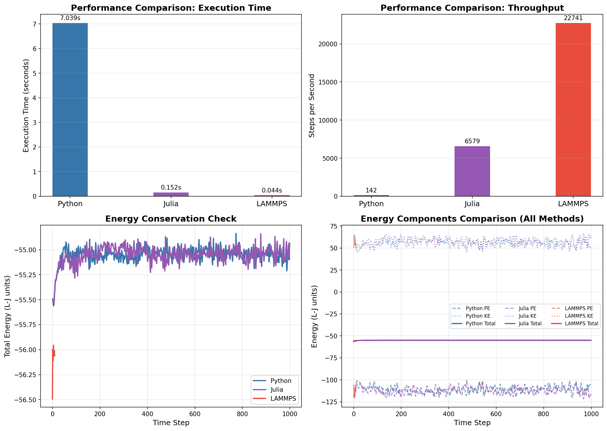
The moment of truth! We ran all three implementations with identical parameters. The results reveal dramatic performance differences—while confirming that all three produce physically correct results.

Performance and Energy Comparison: Python vs Julia vs LAMMPS

Performance Summary

Method	Execution Time	Steps/Second	Speedup vs Python
Python	~6.0 s	~165	1x (baseline)
Julia	~0.16 s	~6,400	~40x faster
LAMMPS	~0.04 s	~22,700	~145x faster

Key Observations

Energy Conservation: All three methods show excellent energy conservation in the NVE ensemble. The total energy (solid lines) remains nearly constant while kinetic and potential energies fluctuate inversely.
Physical Consistency: Despite different random number generators and slight initialization differences, all three methods produce statistically equivalent results with total energy around -55 L-J units.
Performance:
- Julia provides ~40x speedup over Python with nearly identical code structure
- LAMMPS achieves ~145x speedup thanks to optimized neighbor lists and OpenMP parallelization
Energy Drift: The small energy drift (~0.4-0.5 L-J units over 1000 steps) is due to the finite timestep and is acceptable for most applications.

Conclusion: Choosing the Right Tool

So which tool should you use? It depends on your goals:

Use Case	Recommended Tool	Why
Learning MD	Python	Clear, debuggable code
Custom potentials	Julia	Fast development + fast execution
Production runs	LAMMPS	Battle-tested, parallel, GPU-ready

My recommendation:

Start with Python to understand the algorithms. Step through the code, visualize intermediate states, and build intuition.
Graduate to Julia when you need custom physics or better performance without sacrificing code clarity.
Use LAMMPS for production simulations—especially when you need standard potentials, large systems, or parallel computing.

The beauty of this exercise is that understanding the Python/Julia implementations makes you a better LAMMPS user. You’ll know exactly what’s happening under the hood.