Introduction

Flow around a circular cylinder is perhaps the most celebrated benchmark problem in computational fluid dynamics. Why? Because this deceptively simple geometry produces remarkably complex and beautiful physics—from steady symmetric wakes at low Reynolds numbers to the mesmerizing von Kármán vortex street that forms as flow speeds increase.

This problem has been studied experimentally for over a century, providing reliable data for simulation validation. The periodic vortex shedding, characterized by the Strouhal number, and the resulting forces on the cylinder (drag and lift coefficients) provide clear, quantitative metrics for comparison.

This article tackles this classic problem using three of the most widely used CFD platforms:

The goal is not to crown a “winner”—each tool has its place. Instead, this comparison explores how each platform approaches the same problem, examining workflow, usability, and simulation accuracy.

Problem Definition

Physical Background

When fluid flows around a bluff body like a cylinder, the boundary layer separates from the surface, creating a wake region behind the cylinder. At sufficiently high Reynolds numbers, this wake becomes unstable and vortices are shed alternately from each side—the famous von Kármán vortex street.

The Reynolds number, which governs the flow regime, is defined as:

$$Re = \frac{U_\infty D}{\nu}$$

where:

• $U_\infty$ is the freestream velocity
• $D$ is the cylinder diameter
• $\nu$ is the kinematic viscosity

Benchmark Case Parameters

For this comparison, a 2D laminar flow at Re = 100 serves as the test case—a classic regime that produces periodic, well-defined vortex shedding while remaining computationally tractable.

Note: A simplified fluid with ρ = 1 kg/m³ is used, with viscosity calculated from the target Reynolds number. This is a common approach in CFD benchmarking that eliminates material property uncertainties.

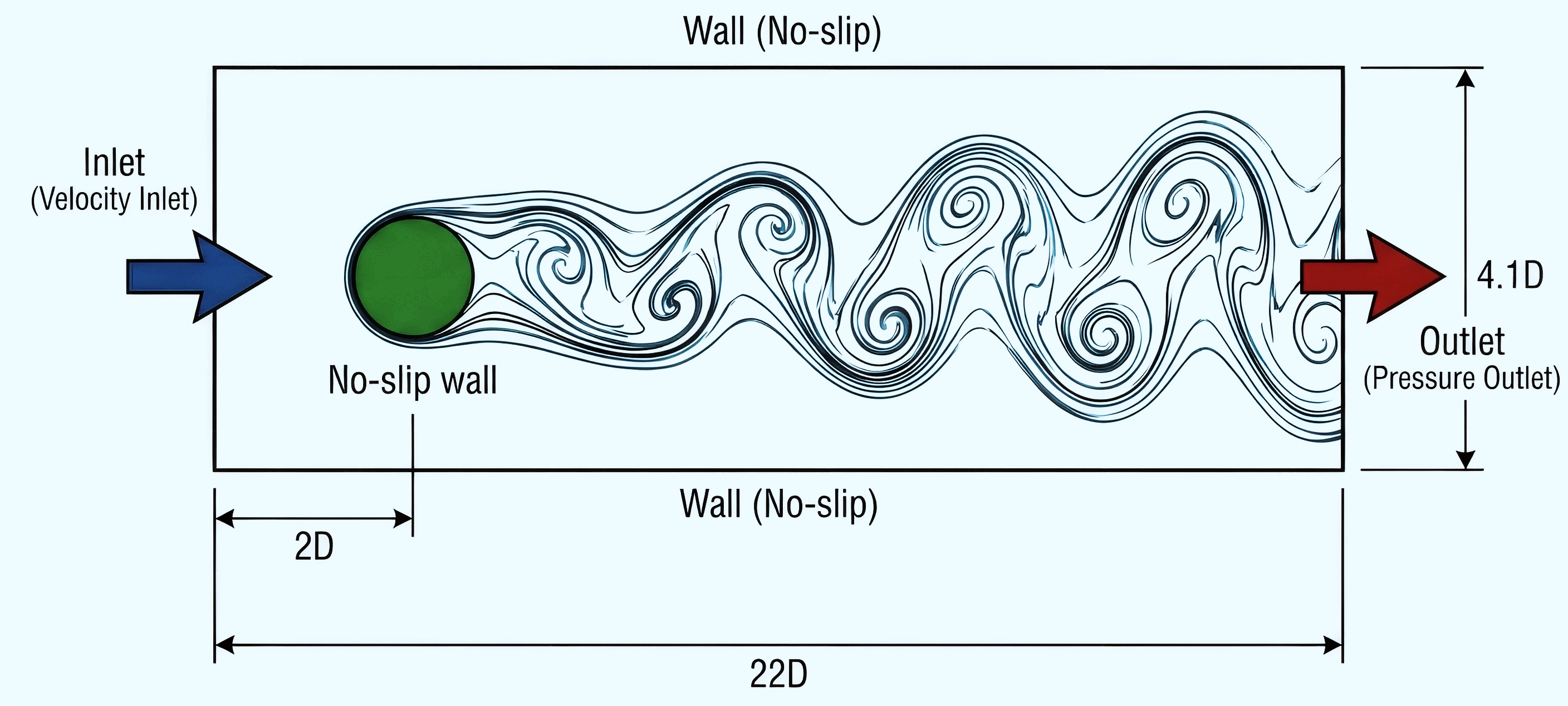
Computational Domain

The domain size significantly affects solution accuracy. A domain that’s too small can artificially constrain the wake development.

Why 4.1D instead of 4D? The domain uses H = 0.41 m with the cylinder centered at y = 0.2 m, creating a slight vertical asymmetry (0.20 m to bottom vs 0.21 m to top). This geometric asymmetry naturally triggers vortex shedding without requiring artificial perturbations, ensuring reproducible results across different solvers.

Governing Equations

The incompressible Navier-Stokes equations govern the flow:

Continuity (mass conservation): $$\nabla \cdot \mathbf{u} = 0$$

Momentum conservation: $$\frac{\partial \mathbf{u}}{\partial t} + (\mathbf{u} \cdot \nabla)\mathbf{u} = -\frac{1}{\rho}\nabla p + \nu \nabla^2 \mathbf{u}$$

Boundary Conditions

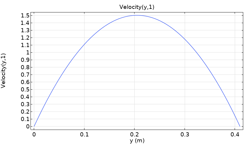
Why a parabolic inlet profile? A fully-developed parabolic (Poiseuille) velocity profile is used at the inlet. The factor of 6 ensures the mean velocity equals $U_m$, while the maximum velocity at the channel center is $1.5 U_m$. This profile represents physically realistic channel flow.

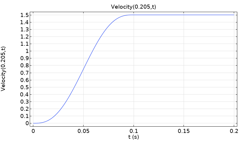
Time ramp-up: In transient simulations, the inlet velocity is multiplied by a smooth step function that ramps from 0 to 1 over the first ~0.1 seconds. This prevents numerical instabilities from an impulsive start and allows the solver to gradually establish the flow field.

Key Performance Metrics

To compare simulation results quantitatively, three well-established metrics are examined:

Why do confined channel values differ? The narrow channel (H = 4.1D) significantly affects the flow. The walls accelerate the fluid around the cylinder (blockage effect), increasing both the effective Reynolds number and forces on the cylinder. The shedding frequency also increases due to the constrained geometry.

COMSOL Multiphysics

Workflow Overview

COMSOL’s physics-first approach makes it intuitive for users familiar with the underlying equations. The workflow follows a logical progression from geometry to results.

flowchart LR
    A[Build\n Geometry] --> B[Define\n Materials]
    B --> C[Add Physics:\n Laminar Flow]
    C --> D[Set Boundary\n Conditions]
    D --> E[Generate\n Mesh]
    E --> F[Configure\n Solver]
    F --> G[Run\n Simulation]
    G --> H[Post-process\n Results]

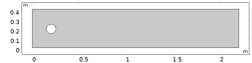
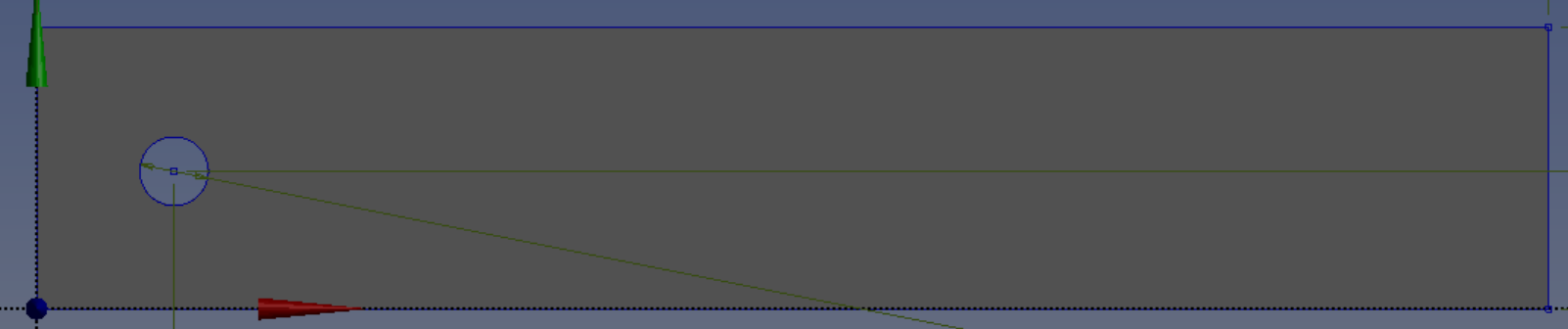
Geometry Setup

In COMSOL, the 2D geometry consists of:

• A rectangular channel domain
• A circular cutout for the cylinder
• Asymmetric cylinder placement to trigger vortex shedding

Physics Configuration

COMSOL uses the Laminar Flow (spf) physics interface:

Boundary Conditions in COMSOL

What is no-slip? The no-slip condition means fluid velocity at a solid surface equals the wall velocity ($\mathbf{u} = 0$ for stationary walls). This physically realistic condition arises from molecular adhesion between fluid and surface, creating the velocity gradients that produce viscous drag.

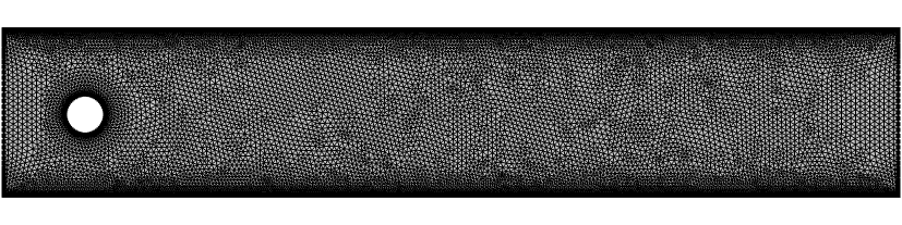
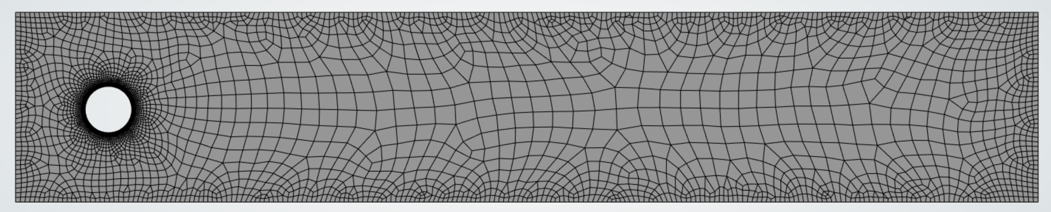
Mesh Strategy

COMSOL’s physics-controlled meshing with manual refinement near the cylinder:

• Free triangular mesh for the domain
• Boundary layers on the cylinder surface (8 layers)
• Size function: Finer near cylinder, coarser in far field
• Maximum element size: 0.1D near cylinder, 0.5D in far field

Solver Settings

For time-dependent simulation:

COMSOL Results

COMSOL provides four main result visualizations configured in the model:

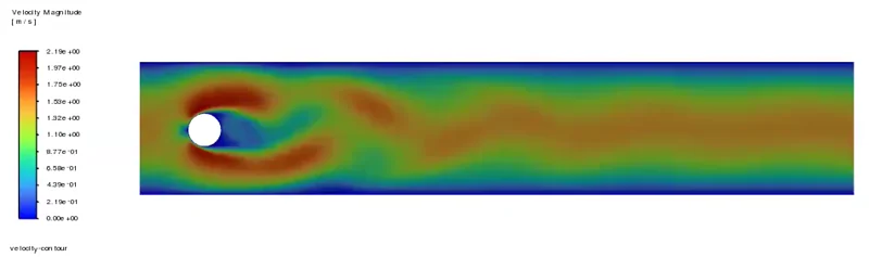
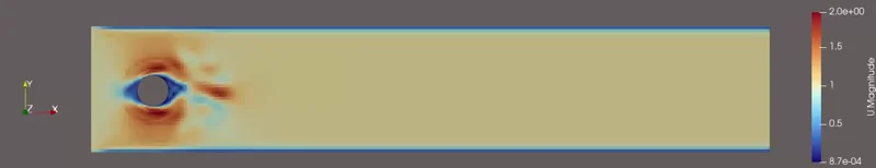
Velocity Field (spf)

The velocity magnitude field shows the development of the von Kármán vortex street behind the cylinder. The animation captures the periodic shedding of alternating vortices.

Pressure Field (spf)

The pressure contours reveal the alternating high and low pressure regions associated with vortex shedding. Note the pressure difference between the front (stagnation) and rear (wake) of the cylinder.

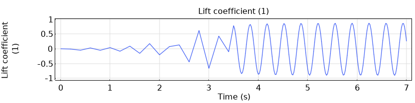
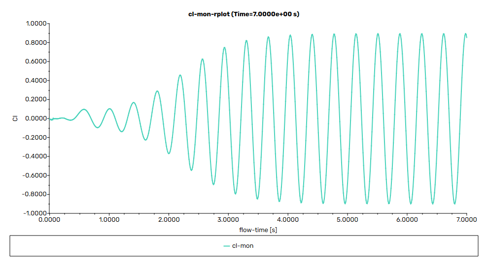
Lift Coefficient

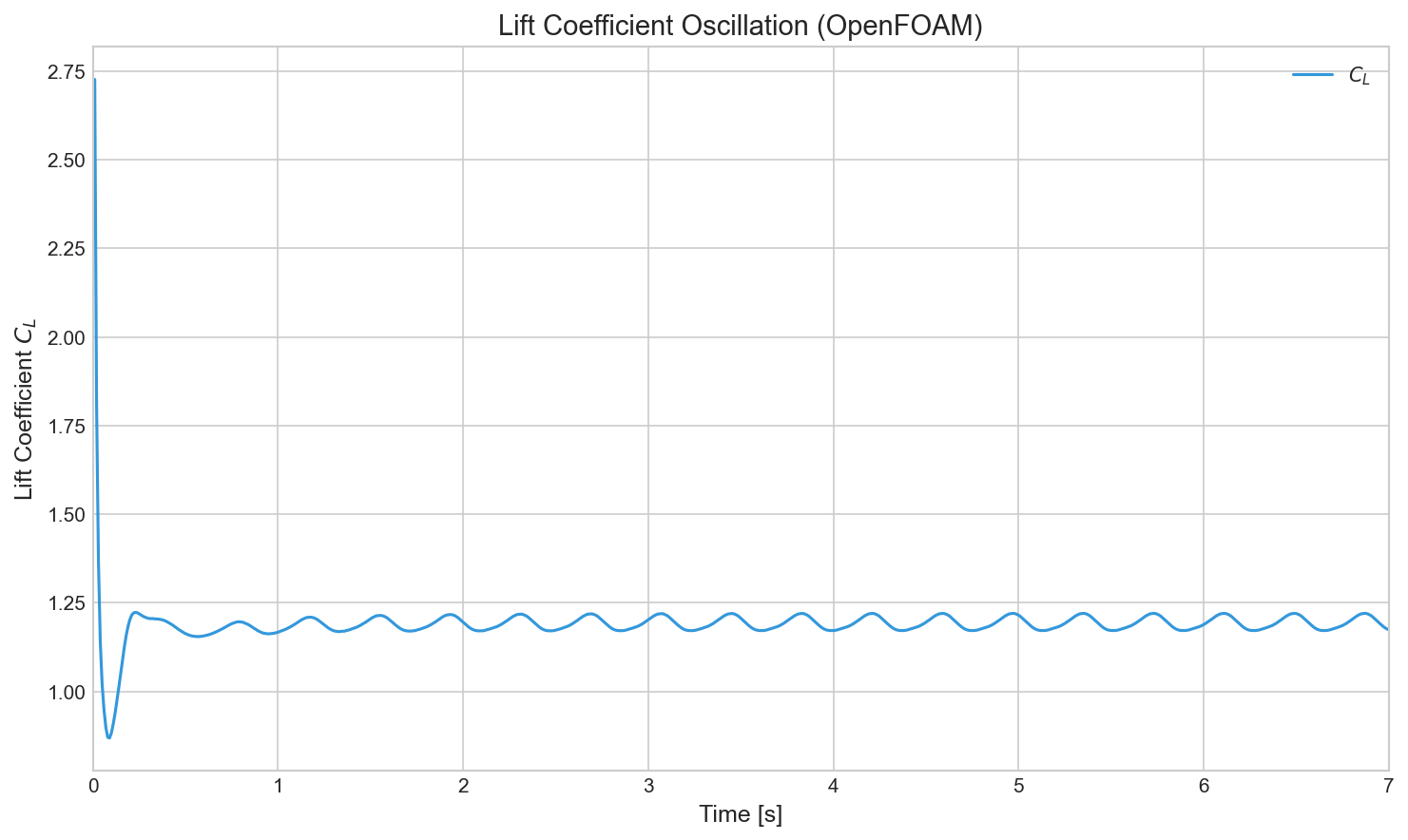
The lift coefficient oscillates periodically once vortex shedding is established. COMSOL calculates it using the expression C_L = -2 × reacf(v) × W / (ρ × U_mean² × D × W), where reacf(v) is the y-component of the reaction force on the cylinder surface.

Drag Coefficient

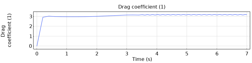
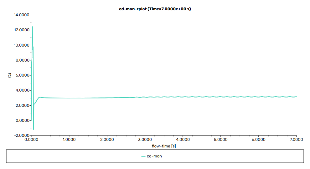
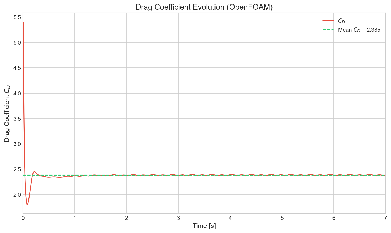
The drag coefficient shows a mean value with small oscillations at twice the shedding frequency. The expression C_D = -2 × reacf(u) × W / (ρ × U_mean² × D × W) uses reacf(u), the x-component of the reaction force.

Strouhal Number Calculation

The Strouhal number is extracted from the lift coefficient oscillation frequency by measuring the period between peaks:

$$St = \frac{f \cdot D}{U_{mean}} = \frac{D}{T \cdot U_{mean}}$$

From the simulation results:

Note: The Strouhal number (St ≈ 0.29) is higher than the classical unbounded flow value (St ≈ 0.164) due to the narrow channel geometry. The channel walls (H = 4.1D) accelerate the flow around the cylinder, increasing the effective velocity and shedding frequency compared to an infinite domain.

ANSYS Fluent

Workflow Overview

Fluent uses multiple integrated tools within the ANSYS Workbench environment:

flowchart LR
    A[DesignModeler\n Geometry] --> B[ANSYS\n Meshing]
    B --> C[Fluent\n Setup]
    C --> D[Fluent\n Solution]
    D --> E[Post-Processing]

Key Setup Summary

Geometry (DesignModeler)

Create a 2D Surface Body (critical for 2D CFD) with:

• Rectangular domain: 2.2 m × 0.41 m
• Circular cutout: D = 0.1 m at (0.2, 0.2) m — note the asymmetric placement to trigger vortex shedding

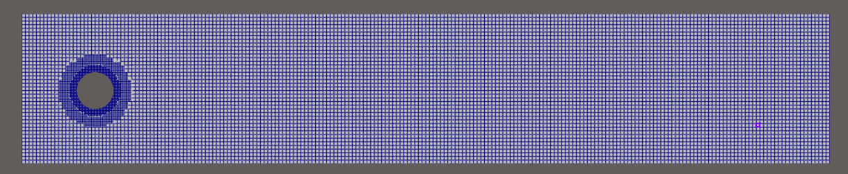
Mesh (ANSYS Meshing)

Physics (Fluent 24R2)

Inlet Boundary (Parabolic Profile)

Fluent supports custom velocity profiles via Expressions:

1

6 [m/s] * y * (0.41 [m] - y) / 0.1681 [m^2] * min(Time / 0.05 [s], 1)

This implements the parabolic profile $u = \dfrac{6 U_m y(H-y)}{H^2}$ with a 0.05s ramp-up, matching the COMSOL configuration.

Solution Method

Monitors

• Drag (cd-mon): Force Report on cylinder, x-direction
• Lift (cl-mon): Force Report on cylinder, y-direction

Fluent Results

OpenFOAM

Workflow Overview

OpenFOAM operates entirely through command-line tools and configuration files:

flowchart LR
    A[blockMesh\n Background Grid] --> B[snappyHexMesh\n Cut Cylinder]
    B --> C[Set BCs\n 0/U, 0/p]
    C --> D[icoFoam\n Solver]
    D --> E[postProcess\n forceCoeffs]
    E --> F[paraFoam\n Visualization]

Case Structure

 1
 2
 3
 4
 5
 6
 7
 8
 9
10
11
12
13
14

openfoam_cylinderFlow/
├── 0/
│   ├── U                    # Velocity (uniform inlet)
│   └── p                    # Pressure
├── constant/
│   └── transportProperties  # ν = 0.001 m²/s
├── system/
│   ├── blockMeshDict        # Background mesh (220×41)
│   ├── snappyHexMeshDict    # Cylinder cutout
│   ├── controlDict          # Solver + forceCoeffs
│   ├── fvSchemes            # Discretization
│   └── fvSolution           # Linear solvers
├── postProcess.py           # Plot generator
└── Allrun                   # Run script

Mesh Generation

Unlike COMSOL/Fluent’s GUI approach, OpenFOAM uses a two-step process:

1. blockMesh: Create rectangular background mesh
2. snappyHexMesh: Cut out the cylinder using implicit geometry

 1
 2
 3
 4
 5
 6
 7
 8
 9
10
11

// snappyHexMeshDict - Cylinder definition
geometry
{
    cylinder
    {
        type    searchableCylinder;
        point1  (0.2 0.2 -0.1);
        point2  (0.2 0.2 0.1);
        radius  0.05;
    }
}

Key Configuration

Transport Properties

1
2

// constant/transportProperties
nu    [0 2 -1 0 0 0 0] 0.001;  // ν = μ/ρ for Re = 100

Force Coefficient Monitoring

 1
 2
 3
 4
 5
 6
 7
 8
 9
10
11
12
13
14
15
16

// system/controlDict - forceCoeffs function
forceCoeffs
{
    type            forceCoeffs;
    libs            (forces);
    patches         (cylinder);
    
    rhoInf          1.0;
    magUInf         1.0;
    lRef            0.1;        // Cylinder diameter
    Aref            0.001;      // D × depth for 2D
    
    liftDir         (0 1 0);
    dragDir         (1 0 0);
    CofR            (0.2 0.2 0);
}

⚠️ Critical: For 2D simulations, Aref = D × mesh_depth = 0.1 × 0.01 = 0.001 m². Using incorrect Aref produces wrong coefficient values.

Running the Simulation

1
2
3
4
5
6
7

# In OpenFOAM environment (Docker/WSL)
blockMesh
snappyHexMesh -overwrite
icoFoam

# Post-processing
python postProcess.py

OpenFOAM Results

Quantitative Results

Why differences? OpenFOAM uses uniform inlet velocity while COMSOL uses parabolic profile. The parabolic profile produces higher velocities at the cylinder height, resulting in stronger vortex shedding and larger force oscillations.

Results Comparison

All three solvers successfully capture the physical phenomena expected at Re = 100:

1. Von Kármán Vortex Street: A stable, periodic shedding of vortices in the wake.
2. Initial Transient: A development phase lasting 2-3 seconds before the periodic regime is established.
3. Oscillatory Forces: Periodic drag and lift forces, with the lift coefficient oscillating at the shedding frequency and drag at twice that frequency.

Differences in absolute numerical values (e.g., peak lift coefficients) include:

• Inlet Profiles: Parabolic (COMSOL) vs. Uniform (OpenFOAM). Parabolic profiles typically result in stronger shedding due to higher centerline velocity.
• Mesh Topology: Unstructured triangular (COMSOL/Fluent) vs. Structured/Hex-dominant (OpenFOAM).
• Time Stepping: Adaptive (COMSOL) vs. Fixed (OpenFOAM).

Despite these configuration differences, the Strouhal number—the dimensionless frequency of vortex shedding—remains consistent across all platforms ($\text{St} \approx 0.28 - 0.29$), confirming the physical validity of each simulation.

Discussion: Workflow & Philosophy

Simulating flow around a cylinder reveals less about the physics—which is constant—and more about the philosophy of each tool. While all three platforms captured the von Kármán vortex street with reasonable accuracy (St ≈ 0.28-0.29), the journey to get there differed significantly.

Workflow Comparison

Conclusion: Choosing the Right Tool

• COMSOL Multiphysics is the Architect’s Choice. Its unified, equation-based interface allowed us to set up the simulation in minutes. It shines when multiphysics coupling is needed.
• ANSYS Fluent is the Engineer’s Workhorse. It offers a balanced ecosystem with powerful meshing tools and robust solvers. It handles complex industrial geometries with ease.
• OpenFOAM is the Researcher’s Scalpel. It demands a steep learning curve but offers unmatched transparency. It is the only choice when you need complete control over every term in the governing equations.

Final Verdict

References

1. Williamson, C. H. K. (1996). “Vortex dynamics in the cylinder wake.” Annual Review of Fluid Mechanics, 28, 477-539.
2. Schäfer, M., Turek, S., et al. (1996). “Benchmark Computations of Laminar Flow Around a Cylinder.” Notes on Numerical Fluid Mechanics, 52, 547-566.
3. Braza, M., Chassaing, P., & Minh, H. H. (1986). “Numerical study and physical analysis of the pressure and velocity fields in the near wake of a circular cylinder.” Journal of Fluid Mechanics, 165, 79-130.
4. COMSOL CFD Module Documentation
5. ANSYS Fluent Theory Guide
6. OpenFOAM User Guide