Introduction

High-Intensity Focused Ultrasound (HIFU) is a non-invasive therapeutic technique that uses acoustic energy to heat and ablate tissue. By focusing ultrasound waves to a small focal region, temperatures can rise rapidly above 60°C, causing coagulative necrosis—a form of controlled tissue destruction used in oncology, neurosurgery, and cosmetic treatments.

This post demonstrates a multi-physics simulation of focused ultrasound heating—combining acoustic wave propagation with bio-heat transfer and thermal dose calculation. The simulation is implemented using two complementary tools:

• k-Wave: An open-source MATLAB toolbox using the k-space pseudospectral method
• COMSOL Multiphysics: A commercial finite element software with multi-physics coupling

Theoretical Background

The Bio-Heat Equation

Tissue heating from ultrasound absorption is governed by the Pennes bio-heat equation:

$$\rho C_p \frac{\partial T}{\partial t} = \nabla \cdot (k \nabla T) + Q$$

where:

• $T$ is the temperature [°C or K]
• $\rho$ is the tissue density [kg/m³]
• $C_p$ is the specific heat capacity [J/(kg·K)]
• $k$ is the thermal conductivity [W/(m·K)]
• $Q$ is the volumetric heat source [W/m³]

In this simulation, we neglect blood perfusion and metabolic heat generation for simplicity.

Acoustic Heat Deposition

The volumetric heat source from acoustic absorption is:

$$Q = \frac{2 \alpha |p|^2}{\rho_0 c_0}$$

where:

• $\alpha$ is the acoustic absorption coefficient [Np/m]
• $p$ is the acoustic pressure amplitude [Pa]
• $\rho_0$ is the tissue density [kg/m³]
• $c_0$ is the sound speed [m/s]

Power Law Absorption

Acoustic absorption in biological tissue follows a power law:

$$\alpha = \alpha_0 f^y$$

where:

• $\alpha_0$ is the frequency-independent absorption coefficient [dB/(MHz^y·cm)]
• $f$ is the frequency [MHz]
• $y$ is the power law exponent (typically 1.0–1.5 for tissue)

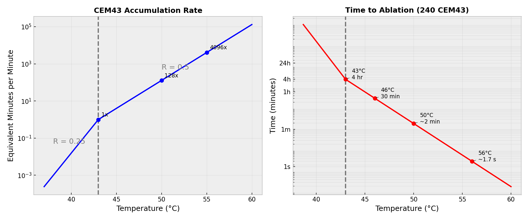
Thermal Dose (CEM43)

Thermal damage is quantified using the Cumulative Equivalent Minutes at 43°C (CEM43):

$$\text{CEM43} = \int_0^{t} R^{43 - T(\tau)} d\tau$$

where:

• $R = 0.5$ for $T \geq 43$°C
• $R = 0.25$ for $T < 43$°C

A CEM43 threshold of 240 minutes is commonly used to define the ablation zone (irreversible tissue damage).

The relationship between temperature and CEM43 accumulation is highly non-linear. The following plot visualizes the accumulation rate and the time required to reach the ablation threshold:

Problem Setup

The simulation models a focused ultrasound transducer heating tissue, with parameters matching the k-Wave example:

Acoustic Parameters

Transducer Geometry

The focused transducer is modeled as a curved arc positioned at the left edge of the domain, focusing ultrasound energy toward the center.

Thermal Parameters

k-Wave Implementation

k-Wave is an open-source MATLAB toolbox that combines efficient acoustic simulation with thermal diffusion capabilities.

Acoustic Simulation

The focused transducer is created using k-Wave’s makeArc function:

1
2
3
4
5
6
7
8
9

% Define transducer arc
source.p_mask = makeArc([Nx, Ny], [1, Ny/2], round(radius/dx), ...
                        round(diameter/dx) + 1, [Nx/2, Ny/2]);

% Define input signal (continuous wave)
source.p = createCWSignals(kgrid.t_array, freq, amp, 0);

% Run acoustic simulation
sensor_data = kspaceFirstOrder2D(kgrid, medium, source, sensor, input_args{:});

The simulation runs until steady state is reached.

Heat Deposition Calculation

After the acoustic simulation reaches steady state, the pressure amplitude is extracted and the heat source is calculated:

 1
 2
 3
 4
 5
 6
 7
 8
 9
10

% Extract pressure amplitude at each position
p = extractAmpPhase(sensor_data.p, 1/kgrid.dt, freq);
p = reshape(p, Nx, Ny);

% Convert absorption to Np/m using power law
alpha_np = db2neper(medium.alpha_coeff, medium.alpha_power) * ...
    (2 * pi * freq).^medium.alpha_power;

% Calculate volume rate of heat deposition
Q = alpha_np .* p.^2 ./ (medium.density .* medium.sound_speed);

Thermal Simulation

The thermal simulation uses k-Wave’s kWaveDiffusion class:

 1
 2
 3
 4
 5
 6
 7
 8
 9
10
11
12
13
14

% Set up diffusion simulation
source.Q = Q;           % heat source
source.T0 = 37;         % initial temperature [°C]

kdiff = kWaveDiffusion(kgrid, medium, source, []);

% Heating phase (10 s)
kdiff.takeTimeStep(round(on_time / dt), dt);
T_after_heating = kdiff.T;

% Cooling phase (source off, 20 s)
kdiff.Q = 0;
kdiff.takeTimeStep(round(off_time / dt), dt);
T_after_cooling = kdiff.T;

k-Wave Results

The acoustic wave animation shows the focused ultrasound field:

The following figure shows the complete simulation results:

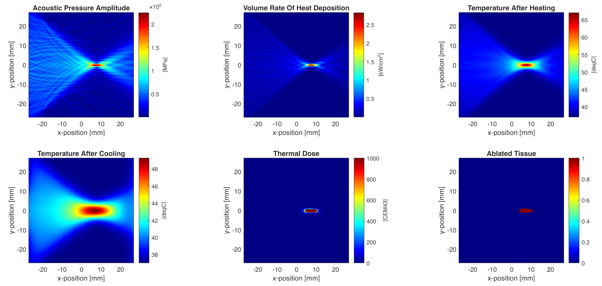
Key observations:

1. Acoustic focusing: The pressure field shows clear focusing at the transducer’s geometric focal point
2. Heat deposition: Concentrated at the focal region where acoustic intensity is highest
3. Temperature rise: Maximum temperature exceeds 60°C at the focus during heating
4. Thermal diffusion: Heat spreads and temperature decreases during cooling
5. Thermal dose: Highest CEM43 values at the focal zone
6. Ablation region: Tissue with CEM43 ≥ 240 min is considered ablated

COMSOL Implementation

COMSOL Multiphysics provides a graphical interface for setting up multi-physics simulations with acoustic-thermal coupling.

Create New Model

1. Open COMSOL Multiphysics 6.4
2. Select Model Wizard → 2D geometry
3. Add physics:
   • Acoustics → Pressure Acoustics, Frequency Domain
   • Heat Transfer → Bioheat Transfer
   • Mathematics → ODE and DAE Interfaces → Domain ODE
4. Select study: Preset Studies → Frequency-Transient

Define Parameters

Go to Global Definitions → Parameters and add:

Build Geometry

1. Right-click Geometry 1 → Rectangle
   • Set size to 54 × 54 mm, centered at origin
2. Right-click Geometry 1 → Parametric Curve
   • Create transducer arc with expressions:
     • x: 35*cos(s)
     • y: 35*sin(s)
   • Parameter range: π - asin(22.5/35) to π + asin(22.5/35) (half-angle calculated from diameter/2 / radius)
   • Position offset: (8, 0) mm (places arc vertex at left boundary)
3. Click Build All

Define Materials

1. Right-click Materials → Blank Material
2. Name it “Tissue” and set:
   • Sound speed: c0
   • Density: rho0
   • Thermal conductivity: k_thermal
   • Heat capacity: cp
3. Assign to domain

Configure Physics

Pressure Acoustics (acpr)

1. Click Pressure Acoustics, Frequency Domain
2. Under Pressure Acoustics Model 1, set:
   • Fluid model: Attenuation
   • Attenuation coefficient: alpha_final
3. Right-click → Pressure → Apply to transducer arc boundaries
   • Set Pressure: amp
4. Right-click → Plane Wave Radiation → Apply to outer boundaries (absorbing BC)

Bioheat Transfer (ht)

1. Right-click Bioheat Transfer → Heat Source
2. Set General source: acpr.Q_pw * rect1(t[1/s])
   • This uses the rect1 function to modulate the acoustic heat source in time (on for 0-10s, off for 10-30s)
3. Set initial temperature: T0

Domain ODE (dode)

1. Configure the dependent variable as cem43_sec
2. Set the source term:

   1 2 3

   // R = 0.5 if T >= 43, else R = 0.25 // Source = R^(43 - T) if(T >= 43[degC], 0.5, 0.25)^((43[degC] - T) / 1[K])

3. This calculates cumulative thermal dose in seconds

Create Rectangle Function

1. Go to Component 1 → Definitions → Functions → Rectangle
2. Set lower limit: 0, upper limit: 10
3. This creates the on/off control for heating

Create Mesh

1. Right-click Mesh 1 → Free Triangular
2. Set Maximum element size to λ/6 ≈ 0.25 mm (wavelength λ = c₀/f₀ = 1.51 mm)
3. Click Build All

Configure Study

1. Step 1: Frequency Domain
   • Set Frequencies: f0
2. Step 2: Time Dependent
   • Set Times: range(0, 0.1, 30)
   • Under Study Extensions, select “Values of variables not solved for” → use solution from Frequency Domain step

Run and Post-Process

1. Click Compute
2. Create Plot Groups:
   • 2D Plot Group 1: Acoustic pressure amplitude
   • 2D Plot Group 2: Heat deposition (acpr.Q_pw)
   • 2D Plot Group 3: Temperature at t = 10 s
   • 2D Plot Group 4: Temperature at t = 30 s
   • 2D Plot Group 5: Thermal dose (cem43_sec / 60)
   • 2D Plot Group 6: Ablated tissue (cem43_sec / 60 >= 240)

COMSOL Results

The acoustic wave animation shows the COMSOL frequency-domain solution:

The COMSOL simulation produces results comparable to k-Wave:

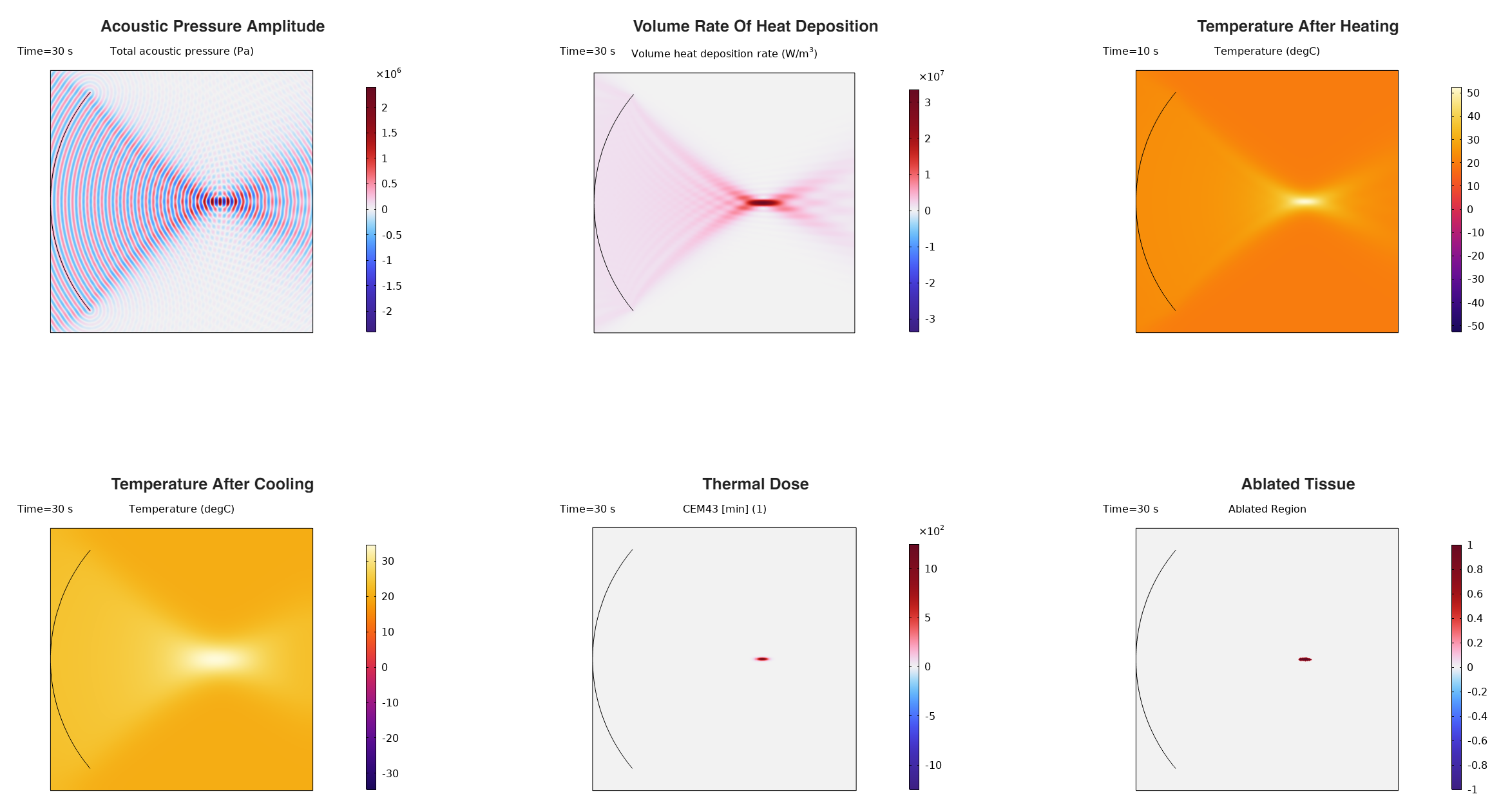
Results Comparison

Visual Comparison

Both simulations show excellent agreement in all physical quantities:

Physical Interpretation

1. Acoustic focusing: The 45 mm diameter transducer with 35 mm focal radius creates a tight focal spot at the domain center
2. Temperature rise: The focal zone reaches temperatures well above 43°C, sufficient for thermal ablation
3. Thermal diffusion: After heating stops, temperature decreases due to thermal conduction, but the ablation has already occurred
4. Lesion formation: The ablated region (CEM43 ≥ 240) is smaller than the peak temperature region, as thermal dose accounts for both temperature and exposure time

Efficiency Comparison

Benchmark Results

*Note: k-Wave timing estimated from acoustic + thermal simulation. Actual timing depends on hardware.

Analysis

1. Mesh/Grid Density: COMSOL uses ~2.7× more elements than k-Wave grid points, as FEM typically requires finer meshes to achieve equivalent accuracy to pseudospectral methods.
2. Acoustic Simulation: k-Wave runs 1,062 time steps to reach steady state, while COMSOL solves directly in frequency domain (single solve). Despite this, the FEM solve is computationally heavier.
3. Thermal Simulation: Both methods use similar time stepping (0.1 s intervals for 30 s), but FEM assembly and solve overhead adds to COMSOL’s computation time.
4. Overall Speedup: k-Wave is approximately 6× faster than COMSOL for this multi-physics simulation.

When to Use Each Tool

Conclusion

Both k-Wave and COMSOL successfully simulate focused ultrasound heating, producing results that agree well with each other. Key findings:

• Multi-physics coupling: Acoustic-thermal simulations require careful coupling of the acoustic pressure field to the thermal heat source
• Thermal dose: CEM43 provides a clinically relevant metric for predicting tissue ablation
• Complementary tools: k-Wave excels in acoustic simulation efficiency, while COMSOL provides integrated multi-physics capabilities

Clinical Relevance

This simulation approach is directly applicable to:

• HIFU therapy planning: Predicting lesion size and shape
• Treatment monitoring: Correlating temperature measurements with thermal dose
• Device design: Optimizing transducer geometry for specific clinical applications

References

1. Treeby, B. E., & Cox, B. T. (2010). k-Wave: MATLAB toolbox for the simulation and reconstruction of photoacoustic wave fields. Journal of Biomedical Optics, 15(2), 021314.
2. Pennes, H. H. (1948). Analysis of tissue and arterial blood temperatures in the resting human forearm. Journal of Applied Physiology, 1(2), 93-122.
3. Sapareto, S. A., & Dewey, W. C. (1984). Thermal dose determination in cancer therapy. International Journal of Radiation Oncology, Biology, Physics, 10(6), 787-800.
4. COMSOL Multiphysics Reference Manual, version 6.4.
5. Duck, F. A. (1990). Physical Properties of Tissue. Academic Press.