What Are We Trying to Do?

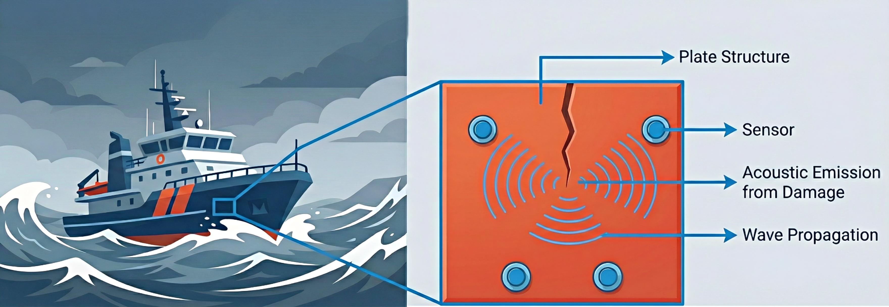
Imagine you’re in a quiet room and someone snaps their fingers. Even with your eyes closed, you can roughly point to where the sound came from. Your brain does this by comparing when the sound reaches each ear—if it hits your right ear first, the source is probably on your right.

Acoustic Emission (AE) source localization works exactly the same way, but for structures like bridges, aircraft panels, or pressure vessels. When materials crack, deform, or break, they release energy as sound waves (ultrasonic waves, actually). By placing sensors on the structure and measuring when each sensor “hears” the sound, we can triangulate where the damage is occurring—often before it becomes visible to the naked eye.

This technique is a cornerstone of Structural Health Monitoring (SHM), helping engineers detect and locate damage in real-time without disassembling anything.

What You’ll Learn

In this article, we’ll walk through:

1. The physics: How sound waves travel through plates (Lamb waves)
2. The math: How to compute source location from arrival time differences (TDOA)
3. The code: A complete, working MATLAB implementation
4. The results: Achieving millimeter-level accuracy in source localization

The Problem Setup

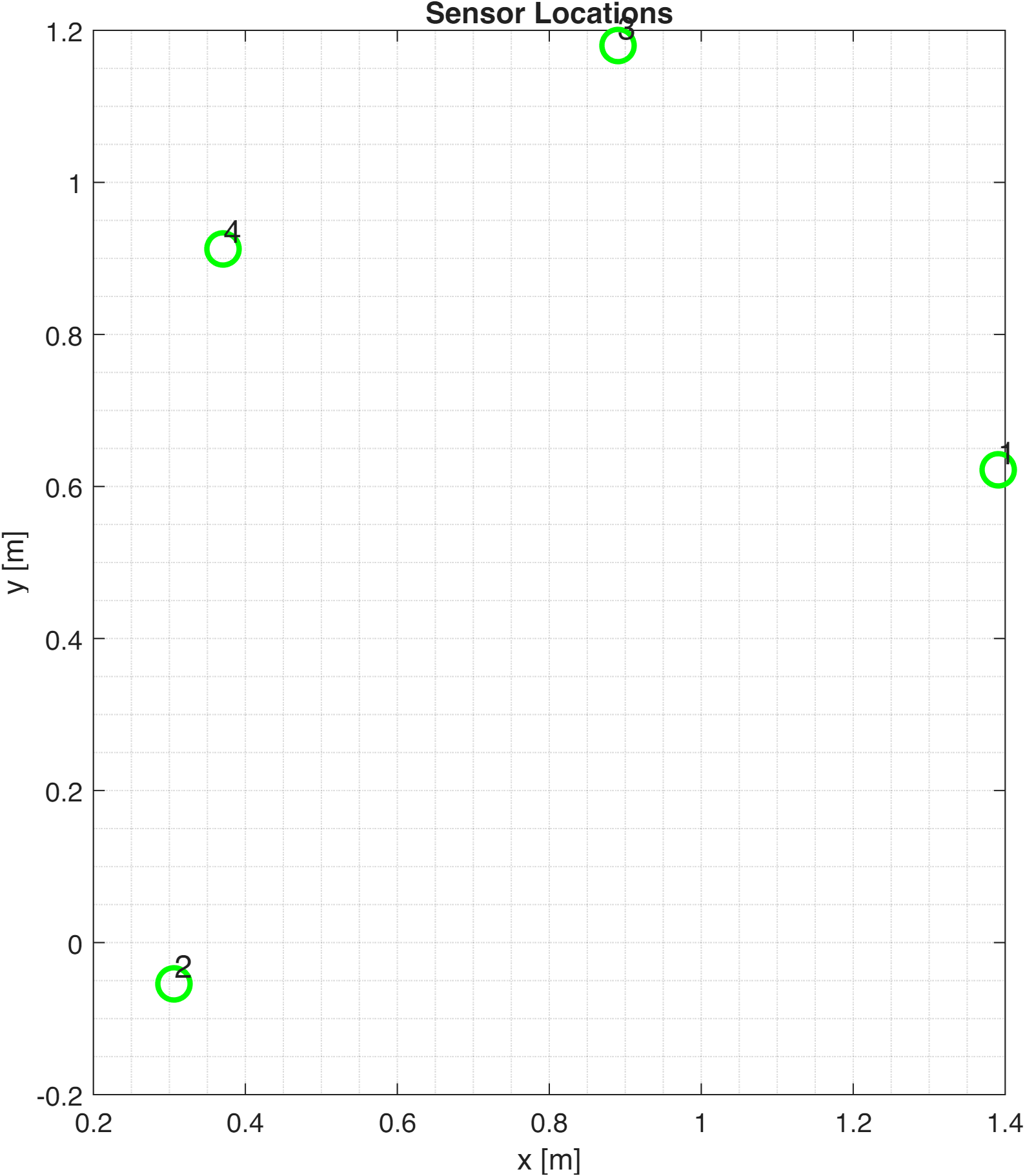
The Sensor Array

We have a metal plate with 4 piezoelectric sensors attached at known locations. These sensors convert mechanical vibrations into electrical signals—think of them as very sensitive microphones for ultrasound.

The Data We Collect

When an acoustic emission event occurs (like a crack forming), each sensor records a time-series signal. Our acquisition system captures:

• Sampling rate: 2 MHz (one sample every 0.5 microseconds—that’s 2 million samples per second!)
• Signal duration: 2.5 milliseconds (5000 samples total)
• Signal units: millivolts (mV)

The Physics: How Sound Travels in Plates

Lamb Waves: Not Your Ordinary Sound Waves

When sound travels through a thin plate (thickness much smaller than wavelength), it doesn’t behave like sound in air. Instead, the waves interact with both surfaces of the plate, creating special wave patterns called Lamb waves.

There are two fundamental types:

The Dispersion Problem

Here’s where it gets tricky: the wave speed changes with frequency. This phenomenon is called dispersion, and it means that different frequency components of your signal travel at different speeds, causing the waveform to “spread out” as it propagates.

$$c_g = c_g(f)$$

For localization purposes, we want to minimize this complication. The S0 mode is our friend here because:

1. ✅ It’s faster (~5300 m/s vs ~1600 m/s) — arrives first, easier to detect
2. ✅ It has weaker dispersion — velocity is more constant across frequencies
3. ✅ The first arrival is cleaner — less interference from reflected waves

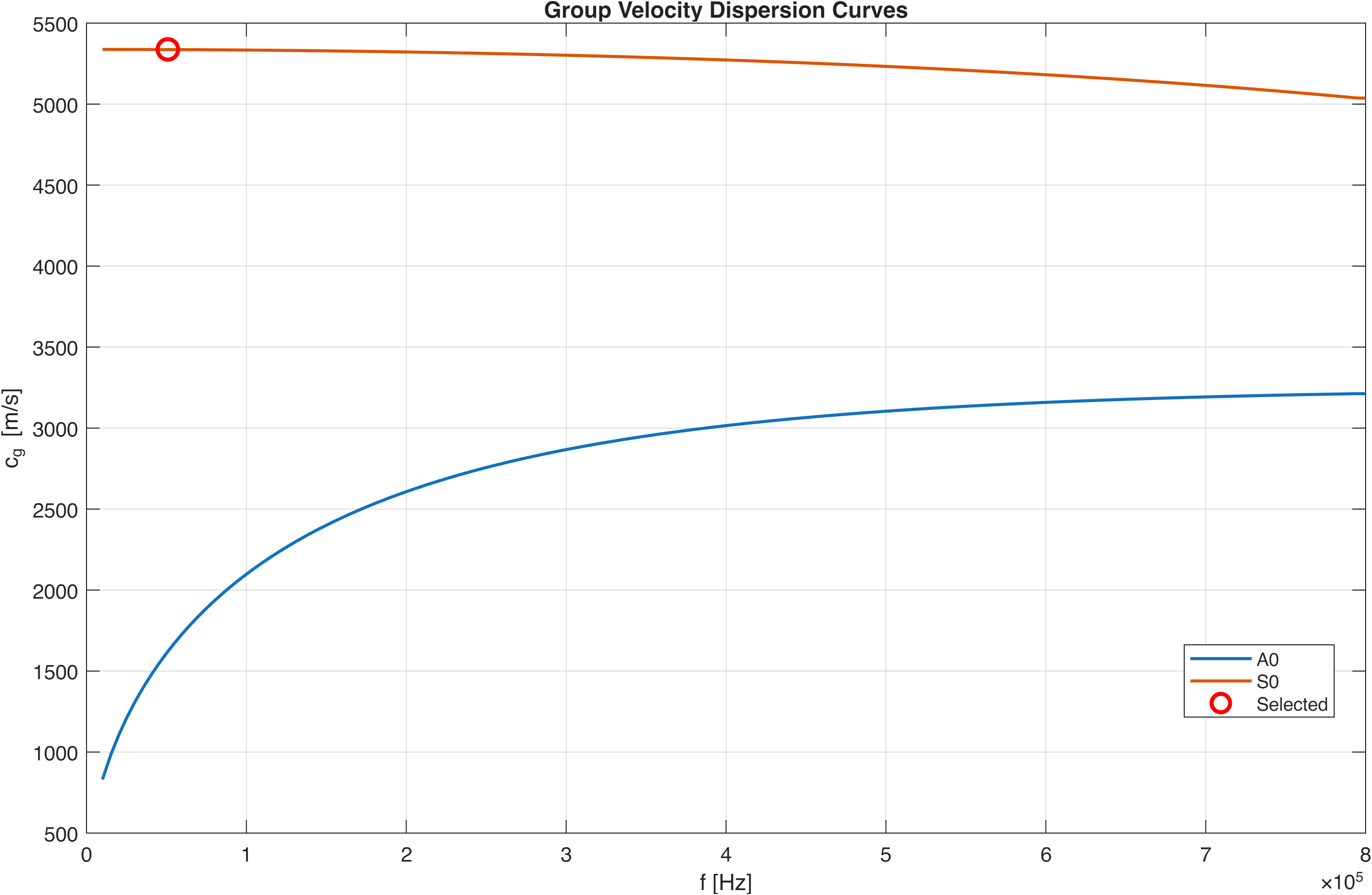
The plot shows how velocity changes with frequency for both modes. Notice how S0 (upper curve) is flatter—less dispersion!

The Algorithm: Time Difference of Arrival (TDOA)

Step 1: Detect When the Wave Arrives

Before we can compare arrival times, we need to accurately determine when the wave hit each sensor. This is called Time of Arrival (TOA) detection.

We use a simple but effective threshold crossing method:

1. Look at the first 100 samples (before the wave arrives) to estimate background noise level
2. Set a threshold at 5× the noise standard deviation
3. The arrival time is when the signal first exceeds this threshold

$$t_{arrival} = \min{t : |s(t)| > 5\sigma_{noise}}$$

Step 2: The TDOA Principle

Now comes the clever part. We don’t actually need to know when the source emitted the wave—we only need to know the differences in arrival times between sensors.

The key insight: If we know:

• The time difference between sensors $i$ and $j$: $\Delta t_{ij} = t_i - t_j$
• The wave speed: $c_g$

Then we can say: the source must lie somewhere such that the difference in distances to the two sensors produces that exact time difference:

$$\frac{d_i - d_j}{c_g} = t_i - t_j$$

Geometrically, all points satisfying this equation form a hyperbola with the two sensors as foci.

Step 3: Combining Multiple Sensor Pairs

With 4 sensors, we have 6 possible pairs: (1,2), (1,3), (1,4), (2,3), (2,4), (3,4).

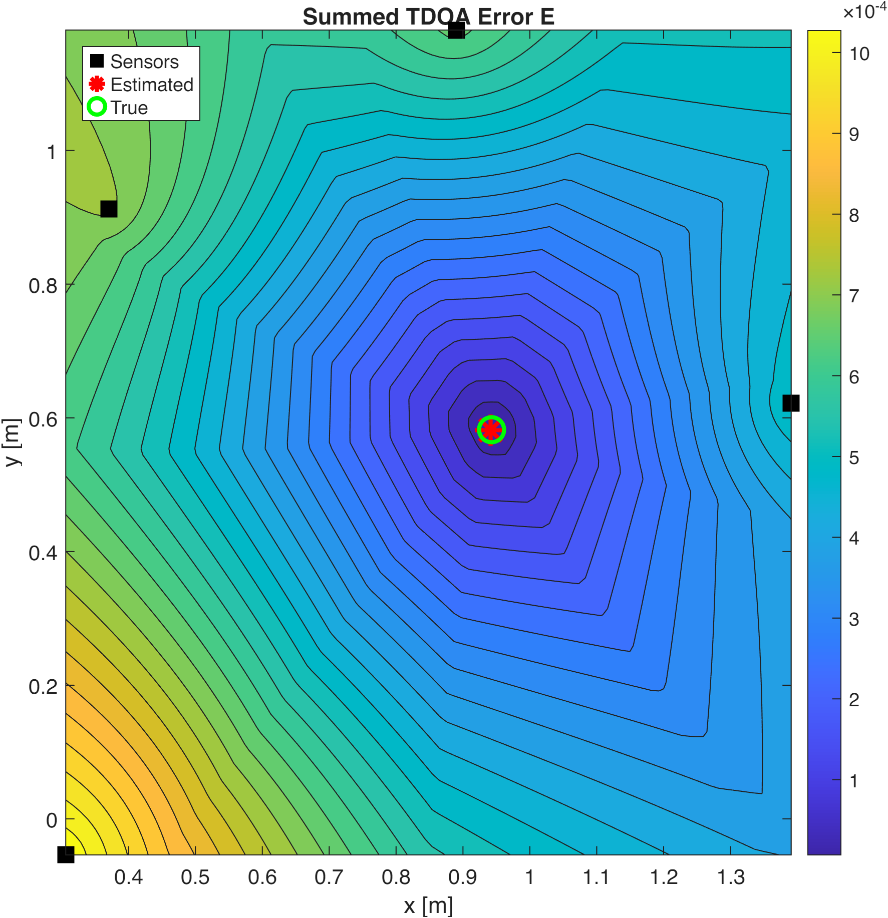
Each pair gives us one hyperbola. The source must lie at the intersection of all these hyperbolas. In practice, due to measurement errors, they won’t intersect at exactly one point—so we define an error function and minimize it.

For each sensor pair $(i, j)$, the error at a hypothetical source position $(x_s, y_s)$ is:

$$E_{ij} = \left| (t_i - t_j) - \frac{d_i - d_j}{c_g} \right|$$

where $d_i = \sqrt{(x_i-x_s)^2 + (y_i-y_s)^2}$ is the distance from source to sensor $i$.

The total error sums all pairs:

$$E = \sum_{i=1}^{3} \sum_{j=i+1}^{4} E_{ij}$$

Goal: Find $(x_s, y_s)$ that minimizes $E$.

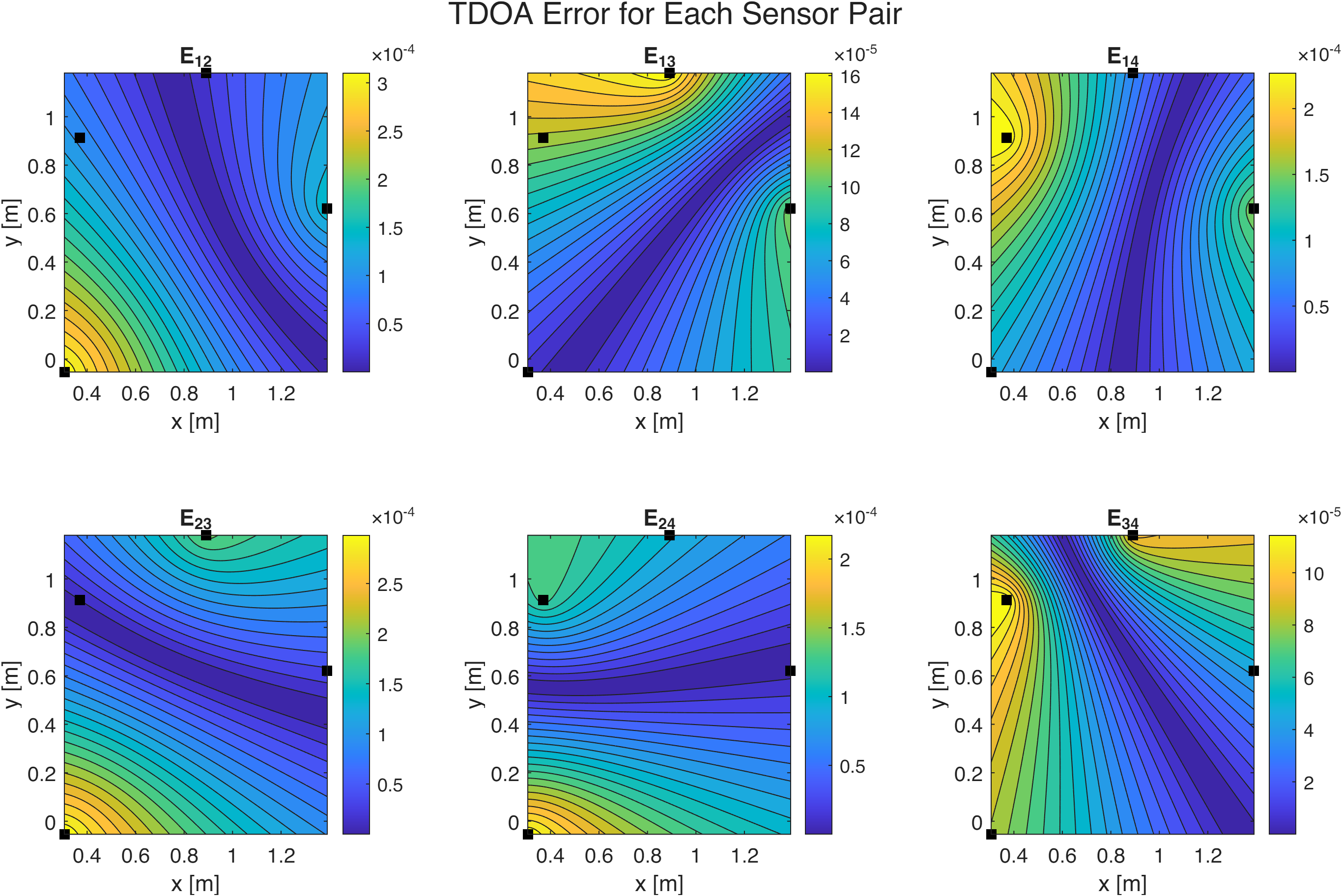
Each subplot shows the error for one sensor pair. Notice the hyperbolic “valleys” (dark blue regions) where the error is low. The source lies where all valleys intersect.

The MATLAB Implementation

Loading and Exploring the Data

 1
 2
 3
 4
 5
 6
 7
 8
 9
10
11
12
13

%% 1. Initialization and Data Loading
clear all; close all; clc;
load('Localisation_exercise_metadata.mat');

% Extract data from the structure
Ex = Metadata;
x = Ex.Isotropic.Coordinates(:,1);  % Sensor X coordinates [m]
y = Ex.Isotropic.Coordinates(:,2);  % Sensor Y coordinates [m]
Grid = Ex.Isotropic.Grid;           % Search grid for localization
s = Ex.Isotropic.Signals;           % Signals [5000 samples × 4 sensors]
t = Ex.Isotropic.Time;              % Time vector [seconds]
f = Ex.Isotropic.Dispersion.f;      % Frequency vector [Hz]
cg = Ex.Isotropic.Dispersion.cg;    % Group velocity [A0; S0]

Detecting Arrival Times

 1
 2
 3
 4
 5
 6
 7
 8
 9
10
11
12
13
14

%% 2. Automatic TOA Detection using Threshold Crossing
toa = zeros(1, 4);           % Initialize arrival times
noise_samples = 100;         % Use first 100 samples for noise estimation

for i = 1:4
    signal = s(:,i);
    noise_level = std(signal(1:noise_samples));  % Noise standard deviation
    threshold = 5 * noise_level;                  % 5× threshold
    first_cross = find(abs(signal) > threshold, 1, 'first');
    toa(i) = t(first_cross);
end

fprintf('Arrival times (μs): %.1f, %.1f, %.1f, %.1f\n', toa*1e6);
% Output: 166.0, 252.0, 195.0, 205.5 μs

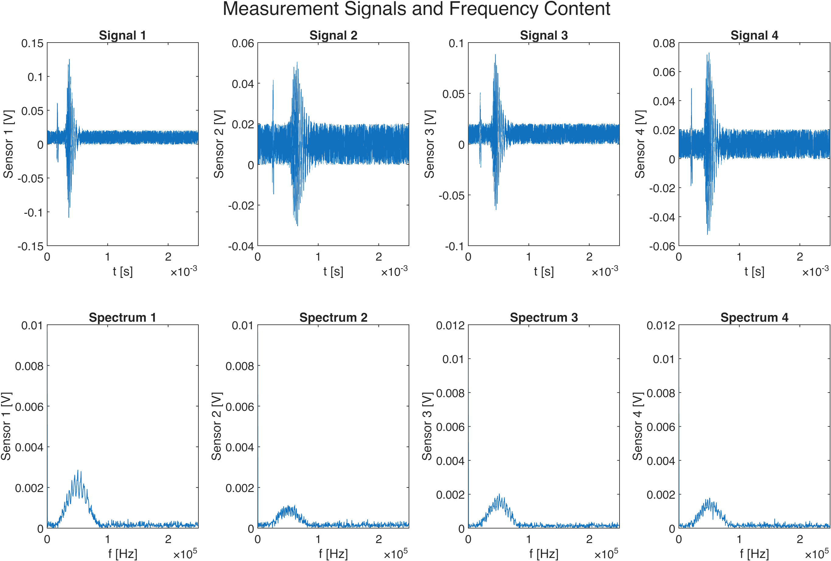
Top row: Time-domain signals from each sensor. Bottom row: Frequency spectra showing energy concentrated around 50 kHz.

Selecting the Wave Velocity

 1
 2
 3
 4
 5
 6
 7
 8
 9
10
11

%% 3. Find Dominant Frequency and Select S0 Mode Velocity
S_avg = mean(S, 2);                            % Average spectrum
min_freq_idx = find(fs > 10000, 1, 'first');  % Skip DC and very low freq
S_avg_search = S_avg;
S_avg_search(1:min_freq_idx-1) = 0;            % Zero out low frequencies
[~, peak_idx] = max(S_avg_search);
dominant_freq = fs(peak_idx);                  % ≈ 51 kHz

% Look up S0 mode velocity at this frequency
[~, freq_idx] = min(abs(f - dominant_freq));
cg_c = cg(2, freq_idx);   % Row 2 = S0 mode; ≈ 5337 m/s

Computing the Error Field and Finding the Source

 1
 2
 3
 4
 5
 6
 7
 8
 9
10
11
12
13
14
15
16
17
18
19
20
21
22
23

%% 4. Calculate TDOA Error Field
E_total = zeros(size(Grid.x));  % Initialize error map

for i = 1:3
    for j = (i+1):4
        % Distance from each grid point to sensors i and j
        dist_i = sqrt((x(i) - Grid.x).^2 + (y(i) - Grid.y).^2);
        dist_j = sqrt((x(j) - Grid.x).^2 + (y(j) - Grid.y).^2);
        
        % TDOA error for this sensor pair
        E_ij = abs((toa(i) - toa(j)) - dist_i/cg_c + dist_j/cg_c);
        E_total = E_total + E_ij;  % Accumulate
    end
end

%% 5. Find the Minimum Error Point
[~, lin_idx] = min(E_total(:));
[row, col] = ind2sub(size(E_total), lin_idx);
x_source = Grid.x(row, col);
y_source = Grid.y(row, col);

fprintf('Estimated source: (%.4f, %.4f) m\n', x_source, y_source);
% Output: Estimated source: (0.9416, 0.5816) m

Results: How Accurate Is This?

That’s remarkably accurate—about the width of a pencil lead!

Where Does the Error Come From?

Summary: The Complete Workflow

1. Collect signals from multiple sensors at known positions
2. Detect arrival times using threshold crossing
3. Analyze spectrum to find dominant frequency
4. Select wave velocity from dispersion curves at dominant frequency
5. Compute TDOA error for all sensor pairs over a spatial grid
6. Find the minimum — that’s your source location!

This workflow achieves millimeter-level accuracy in controlled conditions and forms the foundation for more advanced SHM systems used in aerospace, civil, and mechanical engineering.

Going Further

For beginners: Try modifying the threshold multiplier (currently 5×) and see how it affects the detected arrival times and final accuracy.

For practitioners: Consider implementing:

• Delta-T mapping for better accuracy with limited calibration
• Probabilistic localization to quantify uncertainty
• Machine learning approaches for TOA detection in noisy environments

References

1. EM course: Structural Health Monitoring: Dynamics & Data Analysis, 2025
2. Kundu, T. (2014). Acoustic source localization. Ultrasonics, 54(1), 25-38.
3. Rose, J. L. (2014). Ultrasonic Guided Waves in Solid Media. Cambridge University Press.
4. Baxter, M. G., et al. (2007). Delta T source location for acoustic emission. Mechanical Systems and Signal Processing, 21(3), 1512-1520.