Introduction

Damping is one of the most important yet often misunderstood concepts in mechanical engineering and physics. In simple terms, damping is the mechanism by which a vibrating system loses energy over time. Without damping, a plucked guitar string would vibrate forever, and a car’s suspension would bounce indefinitely after hitting a bump.

Understanding damping is crucial not just for stopping unwanted vibrations, but for designing safer, quieter, and more durable products.

mindmap
  root((Damping))
    Definition
      Energy Dissipation
      Amplitude Decay
      Phase Shift
    Types
      Viscous
      Structural
      Coulomb
      Rayleigh
    Parameters
      Damping Ratio ζ
      Loss Factor η
      Quality Factor Q
    Applications
      Vibration Control
      Shock Absorbers
      Building Dampers

Why Damping Matters

In real-world engineering applications, damping plays a crucial role:

This article provides a comprehensive understanding of damping theory, explores different types of damping, and demonstrates how to simulate damped systems using both Python and COMSOL Multiphysics.

Damping Theory

The Damped Single-Degree-of-Freedom System

The most fundamental model for understanding damping is the Single-Degree-of-Freedom (SDOF) system, consisting of a mass $m$, a spring with stiffness $k$, and a damper with damping coefficient $c$.

The equation of motion is:

$$m\ddot{x} + c\dot{x} + kx = F(t)$$

where:

• $x$ is the displacement
• $\dot{x}$ is the velocity
• $\ddot{x}$ is the acceleration
• $F(t)$ is the external force

For free vibration ($F(t) = 0$) with initial displacement $x_0$, the solution depends on the damping ratio:

$$\zeta = \frac{c}{2\sqrt{km}} = \frac{c}{c_{cr}}$$

where $c_{cr} = 2\sqrt{km}$ is the critical damping coefficient.

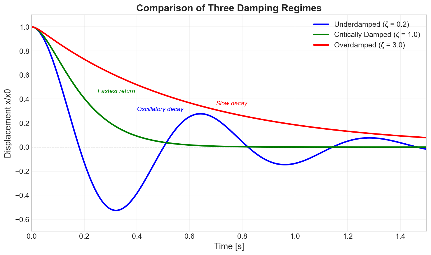
Response Regimes

The system behavior depends entirely on the damping ratio $\zeta$:

For the underdamped case (most common in practice), the free vibration response is:

$$x(t) = x_0 e^{-\zeta\omega_n t} \cos(\omega_d t - \phi)$$

where:

• $\omega_n = \sqrt{k/m}$ is the undamped natural frequency
• $\omega_d = \omega_n\sqrt{1-\zeta^2}$ is the damped natural frequency
• $\phi$ is the phase angle (depends on initial conditions)

Key Insight: The exponential envelope $e^{-\zeta\omega_n t}$ controls how quickly oscillations decay. Higher damping ratio means faster decay.

Types of Damping

Viscous Damping

Viscous damping is the most common mathematical model, where the damping force is proportional to velocity:

$$F_d = -c\dot{x}$$

This model accurately represents:

• Fluid resistance (hydraulic dampers)
• Air drag at low velocities
• Dashpot mechanisms

Energy dissipated per cycle: $$\Delta E = \pi c \omega X^2$$

where $X$ is the amplitude and $\omega$ is the frequency.

Structural (Hysteretic) Damping

Structural damping (also called hysteretic or material damping) occurs due to internal friction within materials. The damping force is proportional to displacement but in phase with velocity:

$$F_d = -\frac{\eta k}{\omega}\dot{x} = -ik\eta x$$

The loss factor $\eta$ is a material property:

Key Property: Energy dissipation is independent of frequency, unlike viscous damping.

Coulomb (Friction) Damping

Coulomb damping arises from dry friction between sliding surfaces:

$$F_d = -\mu N \cdot \text{sgn}(\dot{x})$$

where:

• $\mu$ is the friction coefficient
• $N$ is the normal force
• $\text{sgn}(\dot{x})$ gives the direction opposite to velocity

Characteristics:

• Damping force is constant in magnitude
• Amplitude decreases linearly (not exponentially)
• Motion eventually stops when restoring force < friction force

Rayleigh Damping

Rayleigh damping (or proportional damping) is widely used in finite element analysis. The damping matrix is a linear combination of mass and stiffness matrices:

$$[C] = \alpha[M] + \beta[K]$$

where $\alpha$ (mass-proportional) and $\beta$ (stiffness-proportional) are Rayleigh coefficients.

The damping ratio for mode $n$ is:

$$\zeta_n = \frac{\alpha}{2\omega_n} + \frac{\beta\omega_n}{2}$$

Note: Rayleigh damping is often calibrated using two known frequencies and their damping ratios.

Damping Units and Parameters

Key Parameters and Their Relationships

Relationships Between Parameters

$$\zeta = \frac{\eta}{2} = \frac{1}{2Q} = \frac{\delta}{2\pi}$$

Practical Note: For lightly damped systems ($\zeta < 0.1$), these relationships are approximately valid. For higher damping, use the exact formulas.

Damping Estimation Methods

Logarithmic Decrement Method

From free vibration decay, measure successive peak amplitudes $x_n$ and $x_{n+1}$:

$$\delta = \ln\frac{x_n}{x_{n+1}}$$

The damping ratio is:

$$\zeta = \frac{\delta}{\sqrt{4\pi^2 + \delta^2}}$$

For light damping ($\zeta < 0.1$):

$$\zeta \approx \frac{\delta}{2\pi}$$

Improved accuracy using $n$ cycles:

$$\delta = \frac{1}{n}\ln\frac{x_0}{x_n}$$

Half-Power Bandwidth Method

From a frequency response function, measure the frequency bandwidth $\Delta\omega$ at half-power points (amplitude = peak/$\sqrt{2}$):

$$\zeta = \frac{\Delta\omega}{2\omega_n} = \frac{f_2 - f_1}{2f_n}$$

where $f_1$ and $f_2$ are the frequencies at half-power points.

Curve Fitting Methods

Modern modal analysis software uses curve fitting to extract damping from measured frequency response functions. Common methods include:

• Circle fit (SDOF)
• Line fit (SDOF)
• Polyreference (MDOF)

Effects of Damping

On Free Vibration

Damping causes exponential decay of oscillation amplitude:

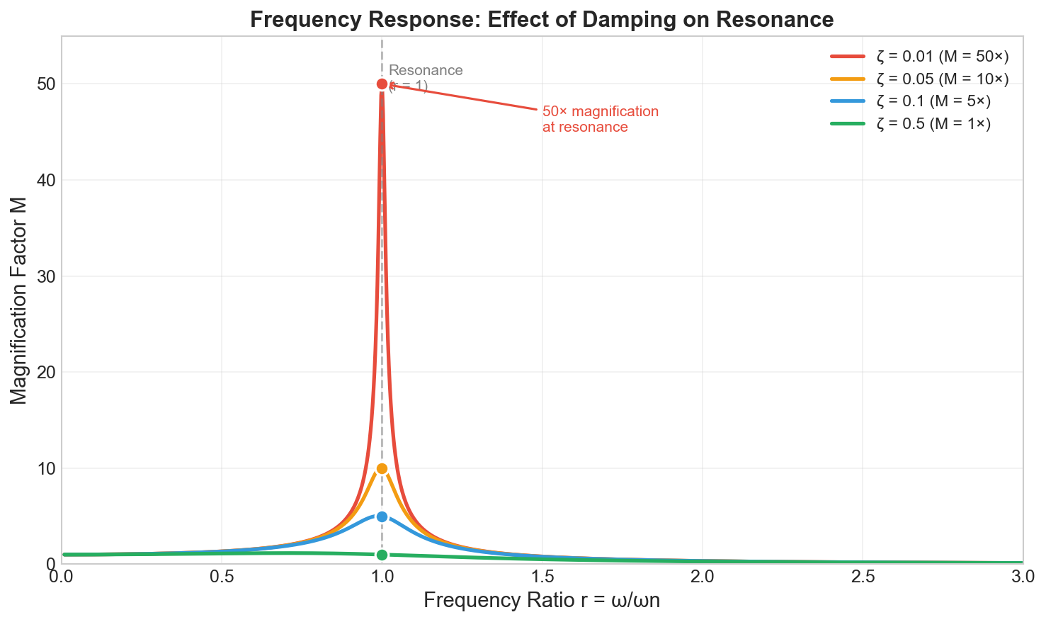
On Forced Vibration

At resonance, the amplitude magnification factor is:

$$M = \frac{1}{2\zeta}$$

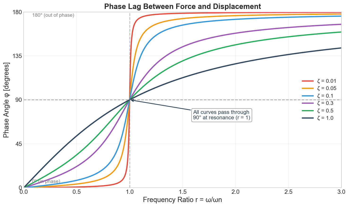
On Phase Shift

The phase angle between force and displacement in forced vibration:

$$\phi = \arctan\frac{2\zeta r}{1 - r^2}$$

where $r = \omega/\omega_n$ is the frequency ratio.

At resonance ($r = 1$), the phase is exactly $90°$ regardless of damping level.

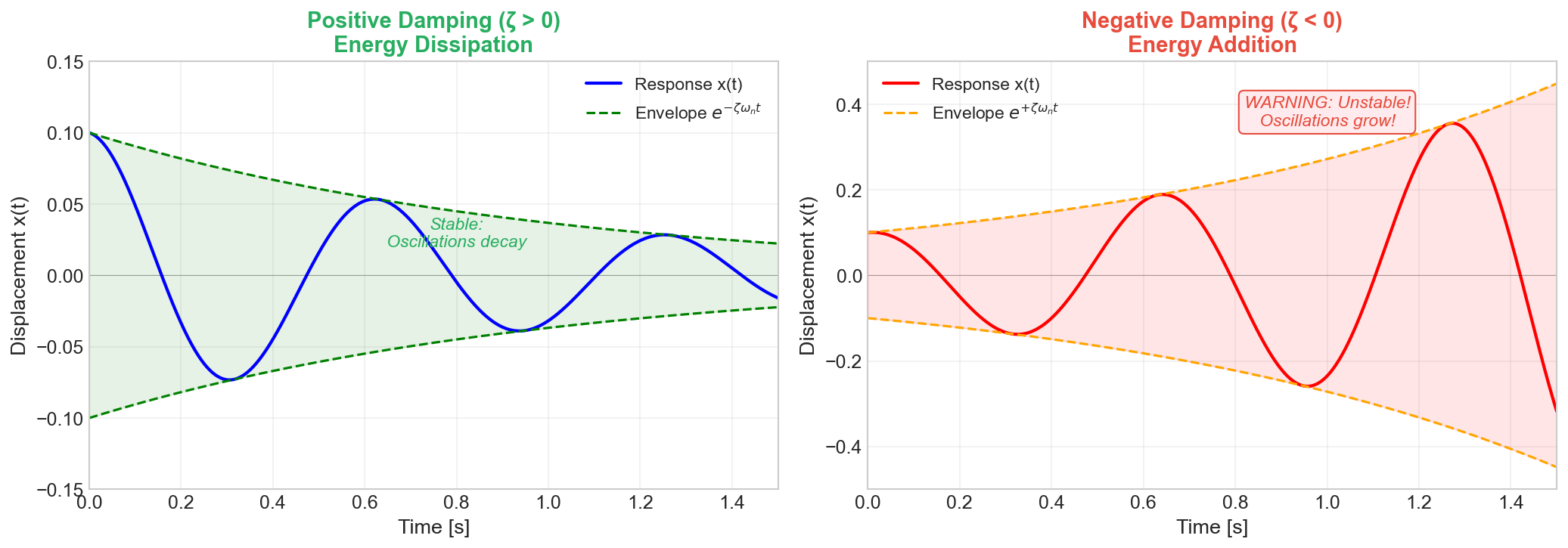
Negative Damping

In certain situations, energy can be added to the system rather than dissipated, leading to negative damping or self-excited oscillations.

Causes of Negative Damping

Mathematical Representation

Negative damping appears as:

$$m\ddot{x} - c\dot{x} + kx = 0$$

The solution grows exponentially:

$$x(t) = x_0 e^{+\zeta\omega_n t} \cos(\omega_d t)$$

Warning: Negative damping leads to unbounded growth unless limited by nonlinear effects.

Case Study: SDOF System Comparison

Let’s compare three approaches to simulate a damped SDOF system:

1. Python (Analytical + Numerical)
2. COMSOL Lumped Mechanical System (ODE solution)
3. COMSOL Physics Field Simulation (Solid Mechanics)

Problem Definition

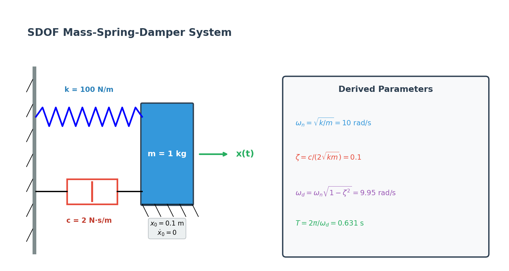
System Parameters:

• Mass: $m = 1$ kg
• Stiffness: $k = 100$ N/m
• Damping ratio: $\zeta = 0.1$ (underdamped)
• Damping coefficient: $c = 2\zeta\sqrt{km} = 2$ N·s/m

Initial Conditions:

• Initial displacement: $x_0 = 0.1$ m
• Initial velocity: $\dot{x}_0 = 0$ m/s

Derived Parameters:

• Natural frequency: $\omega_n = \sqrt{k/m} = 10$ rad/s
• Damped frequency: $\omega_d = \omega_n\sqrt{1-\zeta^2} = 9.95$ rad/s
• Period: $T = 2\pi/\omega_d = 0.631$ s

Method 1: Python Solution

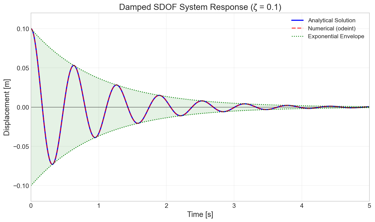
Analytical Solution

For an underdamped system with given initial conditions:

$$x(t) = x_0 e^{-\zeta\omega_n t}\left(\cos\omega_d t + \frac{\zeta}{\sqrt{1-\zeta^2}}\sin\omega_d t\right)$$

Numerical Solution (scipy.integrate.odeint)

 1
 2
 3
 4
 5
 6
 7
 8
 9
10
11
12
13
14
15
16
17
18
19
20
21
22
23
24
25
26
27
28
29
30
31
32
33
34
35
36
37
38
39
40
41
42
43
44
45
46
47
48
49
50
51
52
53
54
55
56
57
58
59
60
61
62
63
64
65
66
67
68
69
70
71
72
73
74
75
76
77
78
79
80
81
82

import numpy as np
from scipy.integrate import odeint
import matplotlib.pyplot as plt

# System parameters
m = 1.0      # mass [kg]
k = 100.0    # stiffness [N/m]
zeta = 0.1   # damping ratio
c = 2 * zeta * np.sqrt(k * m)  # damping coefficient [N·s/m]

# Derived parameters
omega_n = np.sqrt(k / m)  # natural frequency [rad/s]
omega_d = omega_n * np.sqrt(1 - zeta**2)  # damped frequency

# Initial conditions
x0 = 0.1  # initial displacement [m]
v0 = 0.0  # initial velocity [m/s]

# Time array
t = np.linspace(0, 5, 1000)

# Analytical solution for underdamped system (general form with v0)
def analytical_solution(t, x0, v0, zeta, omega_n, omega_d):
    """
    Exact solution for underdamped free vibration.
    x(t) = e^(-ζωn*t) * [A*cos(ωd*t) + B*sin(ωd*t)]
    where A = x0, B = (v0 + ζωn*x0) / ωd
    """
    A = x0
    B = (v0 + zeta * omega_n * x0) / omega_d
    envelope = np.exp(-zeta * omega_n * t)
    return envelope * (A * np.cos(omega_d * t) + B * np.sin(omega_d * t))

# Numerical solution using odeint
def equations(y, t, m, c, k):
    """State-space form: [x, v] -> [dx/dt, dv/dt]"""
    x, v = y
    dxdt = v
    dvdt = (-c * v - k * x) / m
    return [dxdt, dvdt]

y0 = [x0, v0]
solution = odeint(equations, y0, t, args=(m, c, k))
x_numerical = solution[:, 0]

# Analytical result
x_analytical = analytical_solution(t, x0, v0, zeta, omega_n, omega_d)

# Verify both solutions match
max_error = np.max(np.abs(x_analytical - x_numerical))
print(f"Max difference between analytical and numerical: {max_error:.2e} m")

# Plot results
plt.figure(figsize=(10, 6))
plt.plot(t, x_analytical, 'b-', label='Analytical', linewidth=2)
plt.plot(t, x_numerical, 'r--', label='Numerical (odeint)', linewidth=2)
plt.plot(t, x0 * np.exp(-zeta * omega_n * t), 'g:', label='Exponential envelope', linewidth=1.5)
plt.plot(t, -x0 * np.exp(-zeta * omega_n * t), 'g:', linewidth=1.5)
plt.xlabel('Time [s]')
plt.ylabel('Displacement [m]')
plt.title(f'Damped SDOF System Response (ζ = {zeta})')
plt.legend()
plt.grid(True, alpha=0.3)
plt.tight_layout()
plt.savefig('damped_response.png', dpi=150, bbox_inches='tight')
plt.show()

# Calculate logarithmic decrement from peaks
peaks_idx = []
peaks_val = []
for i in range(1, len(x_analytical)-1):
    if x_analytical[i-1] < x_analytical[i] > x_analytical[i+1]:
        peaks_idx.append(i)
        peaks_val.append(x_analytical[i])

if len(peaks_val) >= 2:
    delta = np.log(peaks_val[0] / peaks_val[1])
    zeta_estimated = delta / np.sqrt(4 * np.pi**2 + delta**2)
    print(f"\nLogarithmic decrement: δ = {delta:.4f}")
    print(f"Estimated damping ratio: ζ = {zeta_estimated:.4f}")
    print(f"Actual damping ratio: ζ = {zeta:.4f}")
    print(f"Estimation error: {abs(zeta_estimated - zeta)/zeta * 100:.2f}%")

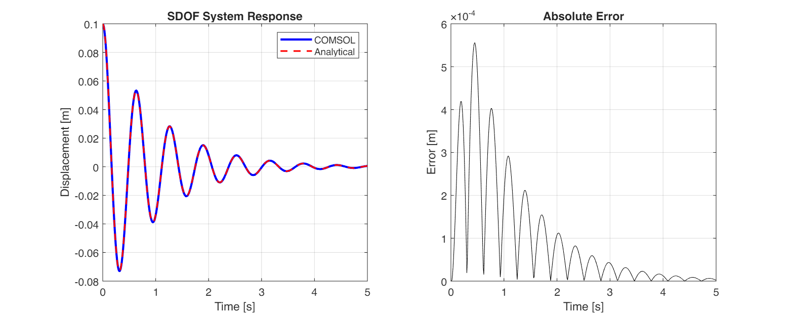
Method 2: COMSOL Lumped Mechanical System

COMSOL’s ODE interface or Lumped Mechanical System can solve the same problem:

Setup Steps:

1. Component → Add Physics → Global ODEs and DAEs
2. Define state variables: x (displacement), v (velocity)
3. Set up equations:
   • d(x,t) = v
   • m * d(v,t) + c * v + k * x = 0
4. Define parameters: m = 1, k = 100, c = 2
5. Set initial values: x(0) = 0.1, v(0) = 0
6. Study → Time Dependent: 0 to 5 s

Method 3: COMSOL Physics Field Simulation

To verify the analytical results within a physical simulation framework (Solid Mechanics), we construct an equivalent 2D mass-spring system that matches the SDOF parameters ($m=1, k=100, c=2$). We use a two-step solver approach to guarantee physically consistent initial conditions:

Setup:

• Geometry: A 2D square with side length $L=0.1$ m and thickness $d=1$ m.
• Material: Effective density $\rho = m/(L^2 d) = 100 \text{ kg/m}^3$ (Total mass = 1 kg).
• Physics (Solid Mechanics 2D):
  • Spring Foundation: Applied to the bottom edge with total stiffness in Y direction $k_{tot} = 100 \text{ N/m}$.
  • Rayleigh Damping: Tuned for equivalent viscous damping ($\alpha_M = 2, \beta_K = 0$).
  • Constraint: Roller constraints on side edges to restrict motion to 1D (vertical).
• Step 1: Stationary Study: Apply a static load $F_{init}$ to pull the mass to $x_0 = 0.1$ m. This computes the precise equilibrium state.
• Step 2: Time Dependent Study: Use the solution from Step 1 as the initial condition, remove the load, and simulate free vibration.

This “Load-Release” method ensures the simulation starts exactly from the analytical initial condition $x(0) = x_0$ with zero initial velocity.

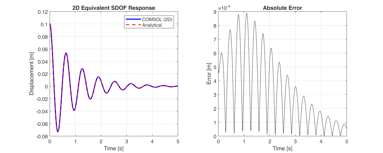
Observation: All methods (Python Analytical, Python Numerical, COMSOL ODE, and COMSOL Solid) produced nearly identical results. The fundamental parameters such as Natural Period ($T \approx 0.631$ s) and Logarithmic Decrement ($\delta \approx 0.632$) matched across all simulations, confirming the validity of the implementation.

Since the macroscopic results are indistinguishable, we focus on the microscopic numerical errors to evaluate the methods:

Note on Numerical Error Comparison:

• For Method 2 (ODE), the error is extremely small (order of $10^{-7}$ m) because it solves the exact differential equation without spatial discretization.
• For Method 3 (FEM), the error is slightly larger (order of $10^{-5}$ m) due to mesh discretization and penalty constraints.

Ideally, the “Absolute Error” line should be zero. Its small non-zero magnitude is the “signature” of numerical approximation, proving the model is working correctly but subject to discrete mathematics.

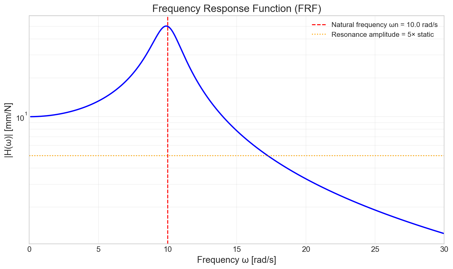
Frequency Response

The frequency response function (FRF) amplitude $H(\omega)$ describes how the system responds to a continuous sinusoidal force at varying frequencies. It reveals the system’s “dynamic stiffness”.

$$H(\omega) = \frac{1}{k}\frac{1}{\sqrt{(1-r^2)^2 + (2\zeta r)^2}}$$

where $r = \omega/\omega_n$.

 1
 2
 3
 4
 5
 6
 7
 8
 9
10
11
12
13
14
15
16

# Frequency response calculation
omega = np.linspace(0.1, 30, 500)
r = omega / omega_n
H = (1/k) / np.sqrt((1 - r**2)**2 + (2*zeta*r)**2)

plt.figure(figsize=(10, 6))
plt.semilogy(omega, H, 'b-', linewidth=2)
plt.axvline(omega_n, color='r', linestyle='--', label=f'ωn = {omega_n} rad/s')
plt.xlabel('Frequency ω [rad/s]')
plt.ylabel('|H(ω)| [m/N]')
plt.title('Frequency Response Function')
plt.legend()
plt.grid(True, alpha=0.3, which='both')
plt.tight_layout()
plt.savefig('frequency_response.png', dpi=150, bbox_inches='tight')
plt.show()

Understanding the Plot: The plot below uses a logarithmic scale (semilog-y) for the amplitude. This is standard in vibration analysis because the response amplitude at resonance can be orders of magnitude larger than at static conditions. A log scale allows us to clearly see both the static response ($H \approx 1/k$) and the sharp resonance peak.

Conclusion

This article has covered the essential aspects of damping in mechanical systems:

1. Damping Theory: The fundamental role of damping in energy dissipation and the characterization through damping ratio $\zeta$.

2. Types of Damping: Viscous, structural, Coulomb, and Rayleigh damping models, each suited for different physical mechanisms.

3. Damping Parameters: The relationships between damping coefficient, damping ratio, loss factor, and quality factor.

4. Estimation Methods: Logarithmic decrement and half-power bandwidth techniques for experimental damping identification.

5. Simulation Comparison: Python and COMSOL approaches produce consistent results for the SDOF benchmark case.

Key Takeaways

Further Reading

• Vibration Fundamentals: Rao, S.S. - Mechanical Vibrations
• Damping Technology: Nashif, A.D. et al. - Vibration Damping
• COMSOL Documentation: Structural Mechanics Module User’s Guide

References

1. Rao, S. S. (2017). Mechanical Vibrations (6th ed.). Pearson.
2. Den Hartog, J. P. (1985). Mechanical Vibrations. Dover Publications.
3. Nashif, A. D., Jones, D. I. G., & Henderson, J. P. (1985). Vibration Damping. John Wiley & Sons.
4. COMSOL Multiphysics Reference Manual. Structural Mechanics Module.
5. Harris, C. M., & Piersol, A. G. (2002). Harris’ Shock and Vibration Handbook (5th ed.). McGraw-Hill.