Learning Objectives

• Understand bias and variance conceptually
• Identify underfitting and overfitting
• Learn strategies to balance model complexity

Theory

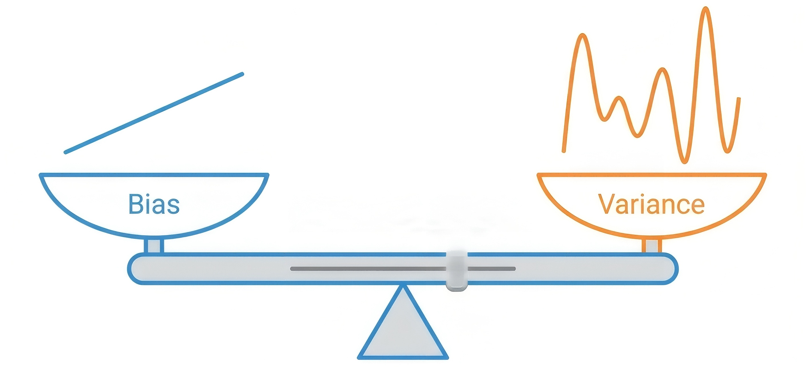
In the previous blog, the generalization bound showed that model complexity affects learning. But what exactly happens when a model is too simple or too complex? This is the bias-variance tradeoff — one of the most important concepts in machine learning.

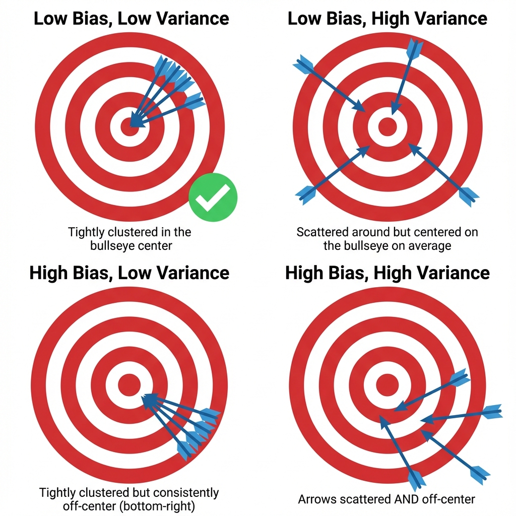
🎯 Archery Analogy: Imagine shooting arrows at a target:

• Bias = How far the average shot lands from the bullseye (systematic error)
• Variance = How spread out the shots are (inconsistency)
• Low bias + Low variance = Tightly clustered shots hitting the bullseye ✅
• High bias + Low variance = Tightly clustered but off-center
• Low bias + High variance = Centered on average but scattered everywhere

Expected Error Decomposition

$$E[(y - \hat{y})^2] = \text{Bias}^2 + \text{Variance} + \text{Irreducible Noise}$$

In plain English: The prediction error comes from three sources:

1. Bias² — The model’s systematic tendency to miss the true value
2. Variance — How much predictions fluctuate across different training sets
3. Noise — Random errors in the data itself (irreducible)

💡 Why Bias² instead of Bias?

• Mathematical necessity: When expanding $E[(y - \hat{y})^2]$, the bias term naturally appears squared
• Non-negative guarantee: Bias can be positive (overestimate) or negative (underestimate), but error contributions must be ≥ 0
• Back to archery: If we didn’t square the bias, shots 5cm left and 5cm right would “cancel out” — clearly wrong for measuring error!

Underfitting vs Overfitting

The following diagram shows how model complexity relates to bias and variance:

The Tradeoff Curve

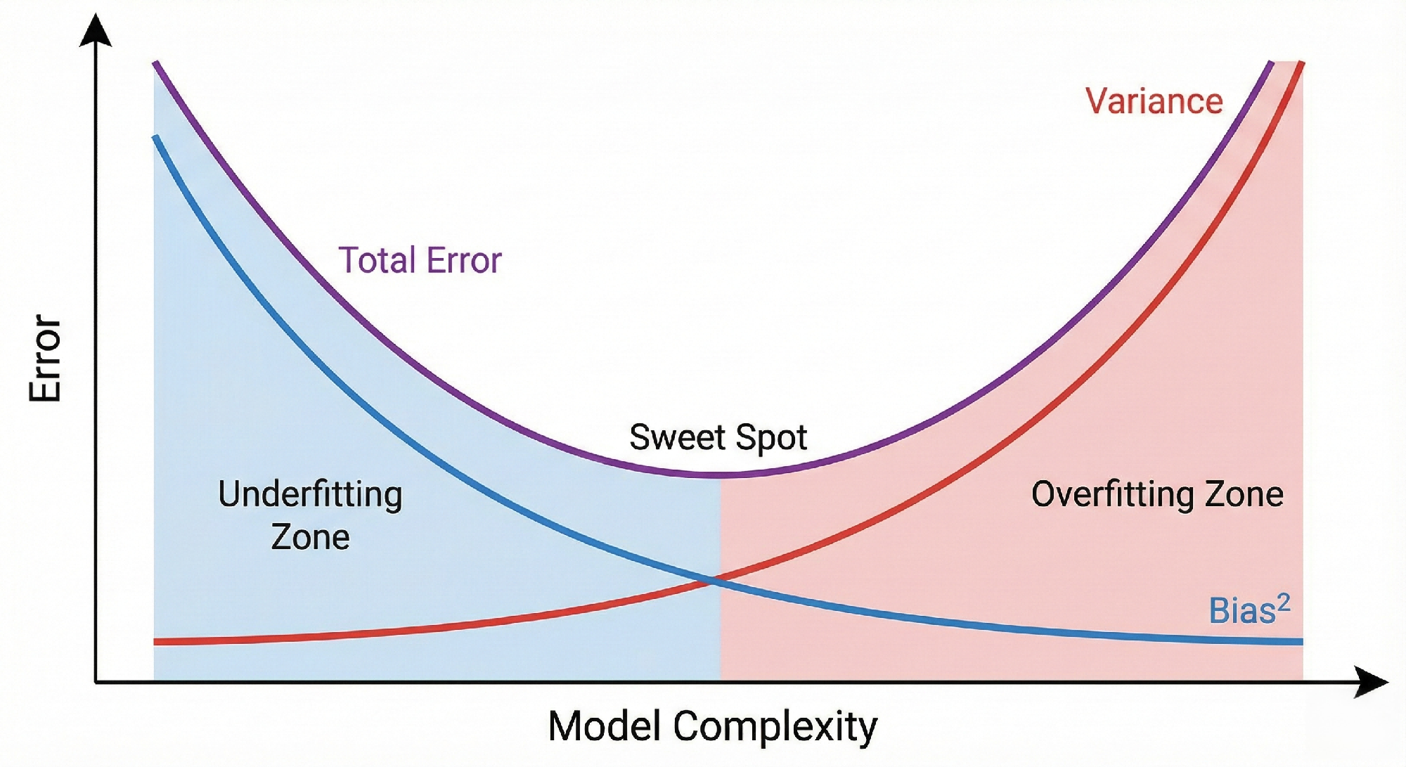
Reading the curve:

• Left side (low complexity): High bias dominates — model is too rigid to capture patterns
• Right side (high complexity): Variance dominates — model is too sensitive to noise
• Minimum point (sweet spot): Optimal complexity where total error is minimized
• Key insight: The curves move in opposite directions — reducing one tends to increase the other

Visual Example

Let’s see this tradeoff in action with polynomial regression on a sine wave:

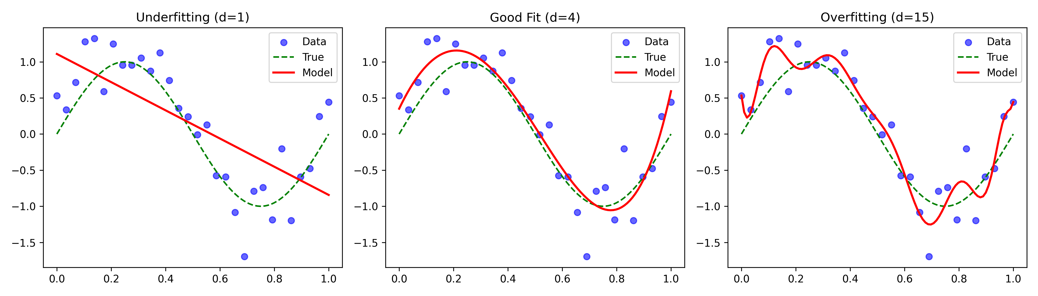
• Degree 1 (Linear): Underfitting — misses the curve
• Degree 4: Just right — captures pattern
• Degree 15: Overfitting — fits noise

Code Practice

Visualizing Bias-Variance

 1
 2
 3
 4
 5
 6
 7
 8
 9
10
11
12
13
14
15
16
17
18
19
20
21
22
23
24
25
26
27
28
29
30
31
32

import numpy as np
import matplotlib.pyplot as plt
from sklearn.preprocessing import PolynomialFeatures
from sklearn.linear_model import LinearRegression

np.random.seed(0)
X = np.linspace(0, 1, 30).reshape(-1, 1)
y_true = np.sin(2 * np.pi * X).ravel()
y = y_true + np.random.normal(0, 0.3, 30)

fig, axes = plt.subplots(1, 3, figsize=(14, 4))
degrees = [1, 4, 15]
titles = ['Underfitting (d=1)', 'Good Fit (d=4)', 'Overfitting (d=15)']

X_plot = np.linspace(0, 1, 100).reshape(-1, 1)

for ax, d, title in zip(axes, degrees, titles):
    poly = PolynomialFeatures(d)
    X_poly = poly.fit_transform(X)
    X_plot_poly = poly.transform(X_plot)
    
    model = LinearRegression().fit(X_poly, y)
    y_plot = model.predict(X_plot_poly)
    
    ax.scatter(X, y, c='blue', alpha=0.6, label='Data')
    ax.plot(X_plot, np.sin(2*np.pi*X_plot), 'g--', label='True')
    ax.plot(X_plot, y_plot, 'r-', linewidth=2, label='Model')
    ax.set_title(title)
    ax.legend()

plt.tight_layout()
plt.savefig('assets/bias_variance.png', dpi=150)

Computing Bias and Variance

 1
 2
 3
 4
 5
 6
 7
 8
 9
10
11
12
13
14
15
16
17
18
19
20
21
22
23
24
25
26
27
28
29
30

from sklearn.model_selection import train_test_split

def bias_variance_simulation(degree, n_simulations=100):
    predictions = []
    
    for _ in range(n_simulations):
        # Generate new dataset
        X = np.random.uniform(0, 1, 50).reshape(-1, 1)
        y = np.sin(2*np.pi*X).ravel() + np.random.normal(0, 0.3, 50)
        
        poly = PolynomialFeatures(degree)
        X_poly = poly.fit_transform(X)
        
        model = LinearRegression().fit(X_poly, y)
        
        X_test = np.array([[0.5]])
        X_test_poly = poly.transform(X_test)
        predictions.append(model.predict(X_test_poly)[0])
    
    predictions = np.array(predictions)
    y_true = np.sin(2 * np.pi * 0.5)
    
    bias = np.mean(predictions) - y_true
    variance = np.var(predictions)
    
    return bias**2, variance

for d in [1, 4, 15]:
    bias_sq, var = bias_variance_simulation(d)
    print(f"Degree {d:2d}: Bias²={bias_sq:.4f}, Var={var:.4f}, Total={bias_sq+var:.4f}")

Output:

1
2
3

Degree  1: Bias²=0.0000, Var=0.0049, Total=0.0049
Degree  4: Bias²=0.0002, Var=0.0084, Total=0.0086
Degree 15: Bias²=0.0000, Var=0.0279, Total=0.0279

Deep Dive

FAQ

Q1: How do I know if I’m underfitting or overfitting?

Q2: Can I have both low bias and low variance?

Yes! With enough data, you can use complex models without overfitting. Ensemble methods (Blog 14-15) also achieve this by combining multiple models.

Q3: Which is worse: underfitting or overfitting?

Both are bad, but overfitting is more insidious — it looks good on training data, giving false confidence. Underfitting is at least honest about its limitations.

Summary

References

• Hastie, T. et al. “The Elements of Statistical Learning” - Chapter 7
• Abu-Mostafa, Y. “Learning From Data” - Chapter 4
• Stanford CS229: Regularization and Model Selection