Learning Objectives

• Distinguish training error vs generalization error
• Explain the No Free Lunch theorem
• Understand hypothesis space and VC dimension
• Grasp PAC learning framework

Theory

Here’s a fundamental question: Why should a model that performs well on training data also perform well on completely new data it has never seen?

Think about it like studying for an exam:

• Training = Practicing with sample problems
• Testing = Taking the actual exam with new questions

A student who memorizes exact answers to practice problems will fail novel exam questions. But a student who understands underlying concepts will succeed. Machine learning faces the same challenge — and this article explains why learning can work at all, and under what conditions.

Training Error vs Generalization Error

When training a model, two types of errors need to be distinguished:

The Core Challenge: The goal is to minimize $E_{out}$, but only $E_{in}$ can be directly measured and minimized. This creates a fundamental gap that all of machine learning theory tries to bridge.

Analogy: Imagine a hospital evaluating a diagnostic AI:

• $E_{in}$ = Error rate on the 1000 patient records used to train the system
• $E_{out}$ = Error rate on all future patients (the real metric that matters)

The hope is that if the model learns true patterns (not just memorizes training cases), these two errors will be close.

flowchart LR
    subgraph Training["🎯 Training Process"]
        A["📊 Training Data
(N samples)"] --> B["🔧 Learning Algorithm"]
        B --> C["✅ E_in
(measurable)"]
    end
    
    subgraph Reality["🌍 Real World"]
        D["∞ All Possible Data"] --> E["❓ E_out
(unknown)"]
    end
    
    C -.->|"🤞 Hope: E_in ≈ E_out"| E
    
    style C fill:#c8e6c9,stroke:#2e7d32
    style E fill:#ffcdd2,stroke:#c62828
    style Training fill:#e3f2fd,stroke:#1565c0
    style Reality fill:#fff3e0,stroke:#ef6c00

No Free Lunch Theorem

This is one of the most important (and humbling) results in machine learning:

Without making assumptions about the problem, no learning algorithm is better than random guessing.

What does this mean?

• An algorithm that works brilliantly on one problem may fail completely on another
• There is no “universal best” algorithm
• Success requires assumptions: patterns exist, the future resembles the past, etc.

Practical implication: When choosing a model, the decision is implicitly making assumptions about the problem. If a linear model is chosen, the assumption is that the relationship is (approximately) linear. If these assumptions are wrong, the model will fail — guaranteed.

Hypothesis Space

Given the No Free Lunch theorem, what assumptions can help? The first key choice is the hypothesis space.

The hypothesis space $\mathcal{H}$ is the set of all possible models that an algorithm can produce. Think of it as the “menu” of options the algorithm is allowed to choose from.

Examples:

Key insight: The choice of hypothesis space is crucial. If the true pattern isn’t in $\mathcal{H}$, the model cannot learn it perfectly, no matter how much data is available.

The training process searches through $\mathcal{H}$ to find the hypothesis $g$ that best approximates the unknown target function $f^*$.

PAC Learning

Now the question becomes: with a finite hypothesis space, when can learning succeed? This is where PAC learning provides the answer.

Probably Approximately Correct learning provides the theoretical foundation for understanding when machine learning is possible.

The PAC guarantee states:

With high probability $(1-\delta)$, the learned model’s generalization error is close to its training error (within tolerance $\epsilon$).

Mathematically:

$$P[E_{out}(g) \leq E_{in}(g) + \epsilon] \geq 1 - \delta$$

Breaking this down:

• $\epsilon$ = maximum acceptable gap between training and test error
• $\delta$ = probability of failure (typically 0.05 or 0.01)
• $E_{in}(g)$ = training error of learned hypothesis $g$
• $E_{out}(g)$ = generalization error of $g$

In plain English: “With 95% confidence, the test error will be at most $\epsilon$ worse than the training error.”

VC Dimension

PAC learning tells us that learning can work, but how do we measure hypothesis space complexity? Enter the VC dimension.

The VC dimension (Vapnik-Chervonenkis dimension) measures the complexity or expressiveness of a hypothesis space. It answers: “How flexible is this family of models?”

Formal definition: The largest number of points that can be shattered (classified in all possible ways) by the hypothesis space.

What does “shatter” mean?

For $n$ points with binary labels, there are $2^n$ possible labeling patterns. If the hypothesis space can achieve every pattern, it can “shatter” those points.

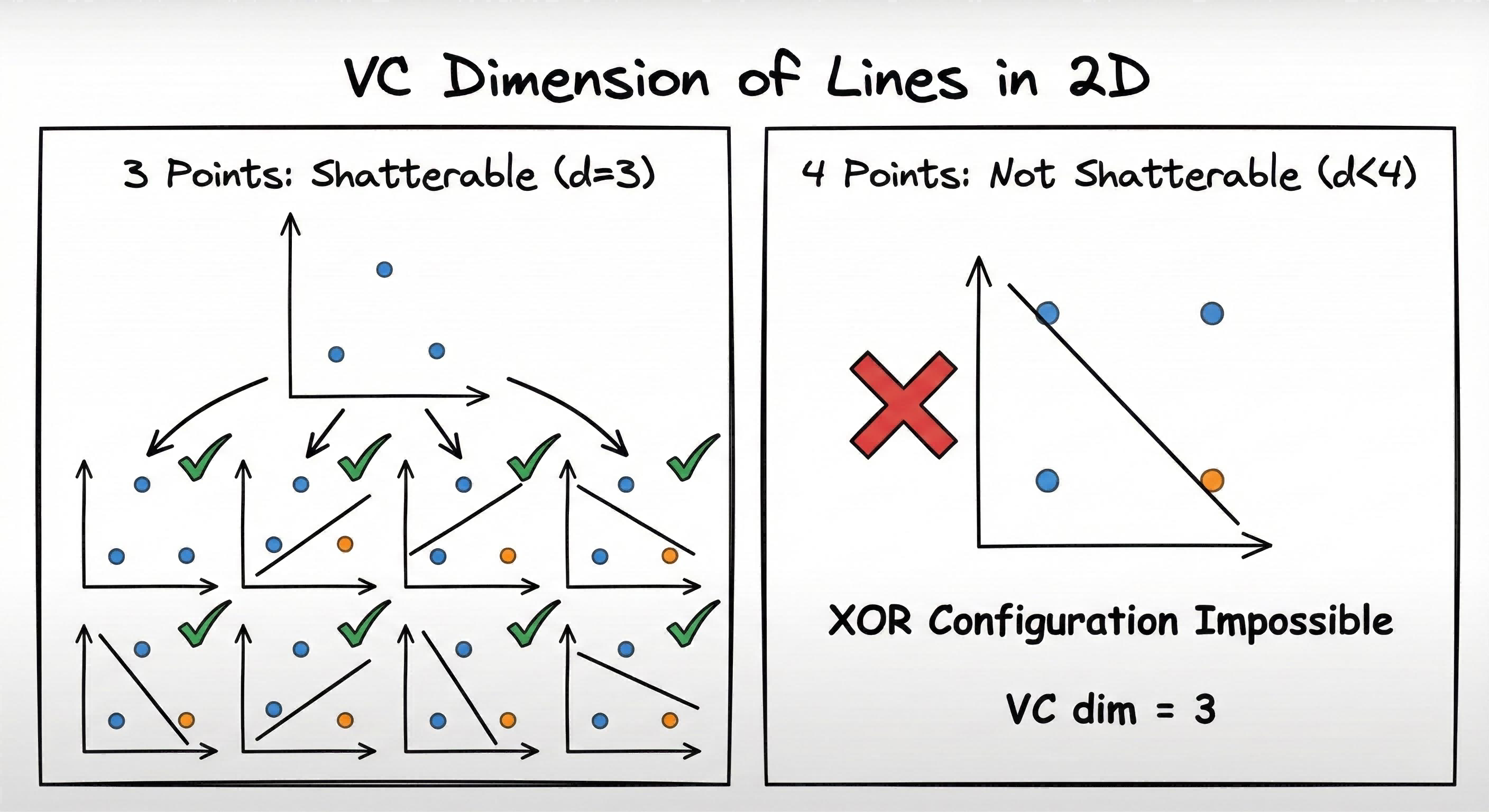
Example: 2D Linear Classifier (Perceptron)

Therefore: $d_{VC} = 3$ for 2D perceptron.

Intuition: Higher VC dimension = more flexible model = can fit more complex patterns, but also more prone to overfitting.

Generalization Bound

This is the central result that explains when machine learning works:

$$E_{out} \leq E_{in} + O\left(\sqrt{\frac{d_{VC}}{N}}\right)$$

Reading this equation:

• Left side: Generalization error (what we care about)
• Right side: Training error + a “complexity penalty”

The penalty term $\sqrt{d_{VC}/N}$ depends on:

💡 Tip: This equation formalizes the bias-variance tradeoff: Complex models (high $d_{VC}$) can achieve low $E_{in}$ but have large penalty. Simple models have small penalty but may have high $E_{in}$. The sweet spot minimizes their sum.

VC Dimension and PAC Learning: The Connection

VC dimension is the key bridge between hypothesis space complexity and PAC learnability:

Fundamental Theorem: A hypothesis space $\mathcal{H}$ is PAC learnable if and only if its VC dimension is finite.

Sample Complexity Bound: The number of samples needed for PAC learning scales with VC dimension:

$$N \geq O\left(\frac{d_{VC} + \ln(1/\delta)}{\epsilon^2}\right)$$

This formula reveals that:

• $d_{VC}$ directly determines the minimum data requirement
• Smaller $\epsilon$ (higher accuracy) requires quadratically more samples
• Smaller $\delta$ (higher confidence) requires logarithmically more samples

Takeaway: Higher VC dimension means more training data is needed to achieve the same $\epsilon$ (accuracy) and $\delta$ (confidence) guarantees. This is why deep neural networks with millions of parameters require massive datasets to generalize well.

Code Practice

The following experiment demonstrates the concepts discussed above in action. It trains polynomial regression models of increasing complexity (degree 1 to 14) and measures both training and test errors.

Training vs Test Error Curve

Experiment setup:

• Generate 100 data points from a sine function with noise
• Split into 70% training, 30% test
• Fit polynomials of degree 1 through 14
• Measure Mean Squared Error on both sets

🐍 Python

1 2 3 4 5 6 7 8 9 10 11 12 13 14 15 16 17 18 19 20 21 22 23 24 25 26 27 28 29 30

import numpy as np from sklearn.preprocessing import PolynomialFeatures from sklearn.linear_model import LinearRegression from sklearn.model_selection import train_test_split from sklearn.metrics import mean_squared_error import matplotlib.pyplot as plt np.random.seed(42) X = np.sort(np.random.uniform(0, 1, 100)).reshape(-1, 1) y = np.sin(2 * np.pi * X).ravel() + np.random.normal(0, 0.2, 100) X_train, X_test, y_train, y_test = train_test_split(X, y, test_size=0.3) degrees = range(1, 15) train_errors, test_errors = [], [] for d in degrees: poly = PolynomialFeatures(d) X_tr_poly = poly.fit_transform(X_train) X_te_poly = poly.transform(X_test) model = LinearRegression().fit(X_tr_poly, y_train) train_errors.append(mean_squared_error(y_train, model.predict(X_tr_poly))) test_errors.append(mean_squared_error(y_test, model.predict(X_te_poly))) plt.plot(degrees, train_errors, 'b-o', label='Train Error') plt.plot(degrees, test_errors, 'r-s', label='Test Error') plt.xlabel('Polynomial Degree'); plt.ylabel('MSE') plt.legend(); plt.yscale('log') plt.savefig('assets/error_curve.png')

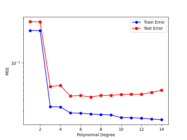
Observation: Training error decreases; test error has a minimum — overfitting!

Interpreting the results:

This is the generalization bound in action: as polynomial degree increases (higher $d_{VC}$), the model becomes more flexible but the complexity penalty grows, eventually dominating.

Deep Dive

FAQ

Q1: Is VC dimension practical or just theoretical?

While computing exact VC dimension is often difficult, it provides crucial intuition: simpler models (lower VC) need less data. In practice, cross-validation is used to empirically estimate generalization.

Q2: What if my training error is already high?

High $E_{in}$ means your model is underfitting — it can’t even capture training patterns. You need a more complex hypothesis space (higher $d_{VC}$).

Q3: How much data do I really need?

Rule of thumb: $N \geq 10 \times d_{VC}$ for reasonable generalization. For neural networks with millions of parameters, this explains why they need massive datasets.

Q4: Why does finite VC dimension guarantee learnability?

Because finite VC bounds the number of “effectively different” hypotheses, making uniform convergence possible. With finitely many distinct behaviors, enough samples ensure that training error approximates generalization error simultaneously for all hypotheses — not just the one selected.

Summary

This article explored the theoretical foundations that explain why machine learning works:

Key Takeaways:

1. Learning works because data comes from a pattern — not random noise
2. Simpler models generalize better when data is limited
3. More data helps by shrinking the generalization gap
4. There’s no free lunch — the right model depends on the problem

References

• Vapnik, V. (1998). “Statistical Learning Theory”
• Abu-Mostafa, Y. et al. “Learning From Data” - Chapters 2-3
• Caltech Machine Learning Course - Lecture 7