ML-06: Linear Regression
Learning Objectives
- Understand regression vs classification
- Derive the least squares solution
- Implement linear regression from scratch
- Extend to multiple features
Theory
Regression vs Classification
| Task | Output Type | Example |
|---|---|---|
| Classification | Discrete labels | Spam or not spam |
| Regression | Continuous values | House price prediction |
Classification answers “which category?” while regression answers “how much?”
Linear Model
$$\hat{y} = w_0 + w_1 x_1 + w_2 x_2 + \cdots = \boldsymbol{w}^T \boldsymbol{x}$$
Where $\boldsymbol{x} = (1, x_1, x_2, \ldots)^T$ includes the bias term (intercept).
Breaking it down:
- $w_0$ is the intercept (baseline prediction when all features are 0)
- $w_1, w_2, \ldots$ are weights that determine how much each feature contributes
- Each weight tells the model: “for every 1-unit increase in this feature, change the prediction by this amount”
Why Squared Error?
The goal is to find the “best” line through data points. What makes a line optimal? Consider these error metrics:
| Error Metric | Formula | Properties |
|---|---|---|
| Sum of errors | $\sum (y_i - \hat{y}_i)$ | ❌ Positive and negative errors cancel out |
| Sum of absolute errors | $\sum \vert y_i - \hat{y}_i \vert$ | ✓ Works, but not differentiable at 0 |
| Sum of squared errors | $\sum (y_i - \hat{y}_i)^2$ | ✓ Differentiable, penalizes large errors more |
Key insight: Squared error is preferred because:
- It’s always positive (no cancellation)
- It’s smooth and differentiable (enables calculus-based optimization)
- It penalizes large errors heavily (one big error is worse than several small ones)
Least Squares Objective
Minimize the sum of squared errors:
$$J(\boldsymbol{w}) = \sum_{i=1}^{N} (y_i - \boldsymbol{w}^T \boldsymbol{x}_i)^2 = |\boldsymbol{y} - X\boldsymbol{w}|^2$$
In matrix form, where $X$ is the design matrix (each row is a sample, each column is a feature):
- $\boldsymbol{y}$ = vector of true values $(y_1, y_2, \ldots, y_N)^T$
- $X\boldsymbol{w}$ = vector of predictions
- $|\cdot|^2$ = squared Euclidean norm
Deriving the Closed-Form Solution
The optimal weights can be derived step by step.
Step 1: Expand the objective function
$$J(\boldsymbol{w}) = (\boldsymbol{y} - X\boldsymbol{w})^T(\boldsymbol{y} - X\boldsymbol{w})$$
Expanding the product:
$$J(\boldsymbol{w}) = \boldsymbol{y}^T\boldsymbol{y} - 2\boldsymbol{w}^T X^T \boldsymbol{y} + \boldsymbol{w}^T X^T X \boldsymbol{w}$$
Step 2: Take the gradient with respect to $\boldsymbol{w}$
Using matrix calculus rules:
- $\frac{\partial}{\partial \boldsymbol{w}}(\boldsymbol{w}^T \boldsymbol{a}) = \boldsymbol{a}$
- $\frac{\partial}{\partial \boldsymbol{w}}(\boldsymbol{w}^T A \boldsymbol{w}) = 2A\boldsymbol{w}$ (when $A$ is symmetric)
$$\nabla_w J = -2X^T\boldsymbol{y} + 2X^T X\boldsymbol{w}$$
Step 3: Set gradient to zero and solve
$$-2X^T\boldsymbol{y} + 2X^T X\boldsymbol{w}^* = 0$$
$$X^T X \boldsymbol{w}^* = X^T \boldsymbol{y}$$
$$\boldsymbol{w}^* = (X^T X)^{-1} X^T \boldsymbol{y}$$
This is the normal equation — a direct, closed-form solution for linear regression.
Geometric Interpretation
The prediction $\hat{\boldsymbol{y}} = X\boldsymbol{w}$ is the projection of $\boldsymbol{y}$ onto the column space of $X$.
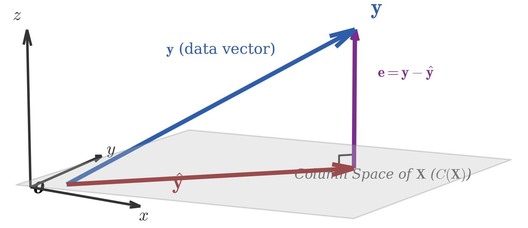
Why projection? The intuition:
- The column space of $X$ contains all possible predictions the model can make
- The true $\boldsymbol{y}$ might not be in this space (data is rarely perfectly linear)
- The closest point in this space to $\boldsymbol{y}$ is its orthogonal projection
- “Closest” in Euclidean distance = minimizing squared error!
The orthogonality condition: The residual vector $(\boldsymbol{y} - \hat{\boldsymbol{y}})$ is perpendicular to every column of $X$:
$$X^T(\boldsymbol{y} - X\boldsymbol{w}) = 0$$
This is exactly the normal equation rearranged—geometry and calculus yield the same answer.
Understanding R² Score
The coefficient of determination ($R^2$) measures how well the model explains the variance in the data:
$$R^2 = 1 - \frac{SS_{res}}{SS_{tot}} = 1 - \frac{\sum(y_i - \hat{y}_i)^2}{\sum(y_i - \bar{y})^2}$$
Where:
- $SS_{res}$ = Residual sum of squares (unexplained variance)
- $SS_{tot}$ = Total sum of squares (total variance)
- $\bar{y}$ = mean of $y$
Interpreting R²:
| R² Value | Interpretation |
|---|---|
| 1.0 | Perfect fit — model explains all variance |
| 0.8 | Good — 80% of variance explained |
| 0.5 | Moderate — half the variance explained |
| 0.0 | Model is no better than predicting the mean |
| < 0 | Model is worse than predicting the mean |
Code Practice
From Scratch Implementation
🐍 Python
| |
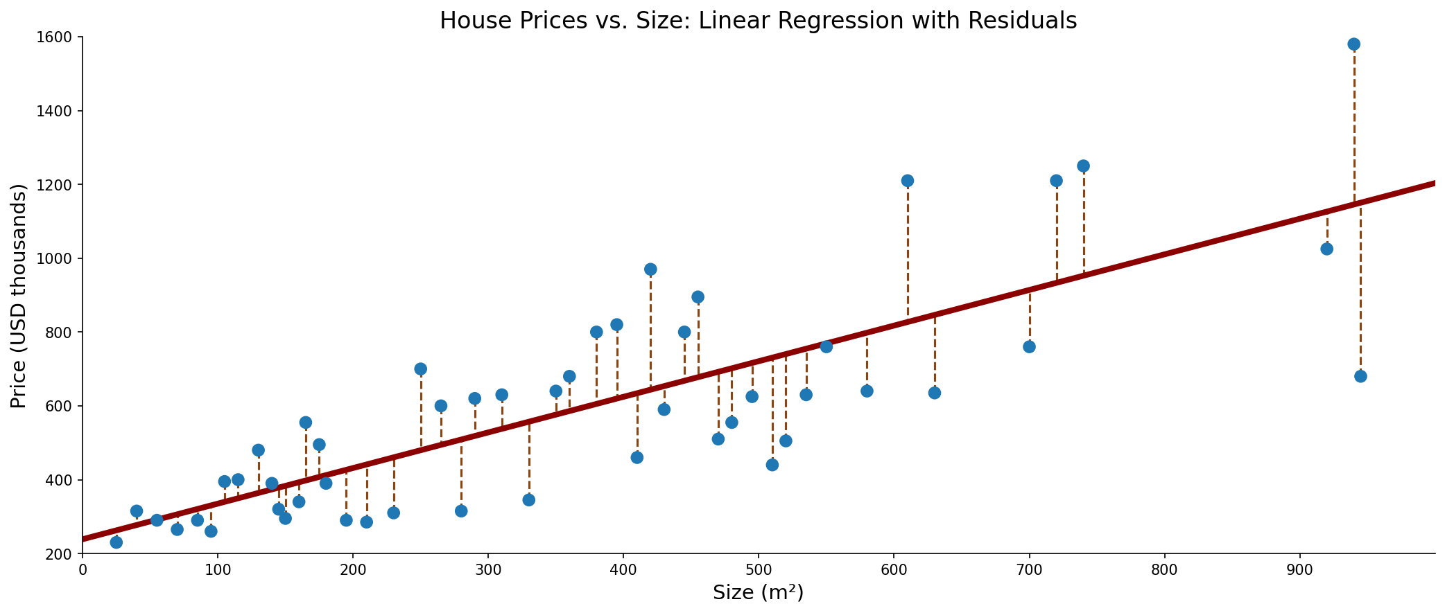
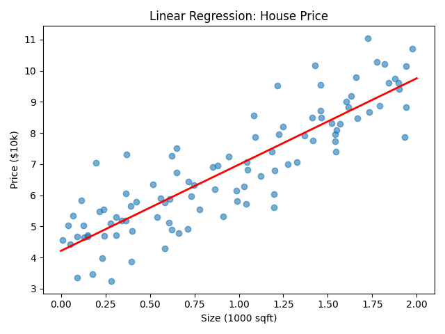
Example: House Price
🐍 Python
| |
Output:
Multiple Linear Regression
🐍 Python
| |
Output:
Deep Dive
Q1: When does the normal equation fail?
The normal equation $\boldsymbol{w}^* = (X^T X)^{-1} X^T \boldsymbol{y}$ requires inverting $X^T X$, which can fail or be problematic in several cases:
| Problem | Cause | Solution |
|---|---|---|
| Singular matrix | Features are linearly dependent (e.g., feature_3 = 2 × feature_1) | Remove redundant features or use regularization |
| Near-singular matrix | Features are highly correlated (multicollinearity) | Use Ridge regression (L2 regularization) |
| Large dataset | Matrix inversion is $O(n^3)$, slow for millions of samples | Use gradient descent (iterative, $O(n)$ per step) |
| More features than samples | $X^T X$ is not full rank when $p > n$ | Use regularization or dimensionality reduction |
Practical rule of thumb: Use normal equation for small datasets (< 10,000 samples), gradient descent for large ones.
Q2: What does a negative coefficient mean?
A negative weight indicates an inverse relationship: as that feature increases, the prediction decreases (holding other features constant).
Examples:
- House prices: “years since renovation” → negative (older renovation = lower price)
- Test scores: “hours of distraction” → negative (more distraction = lower score)
- Fuel efficiency: “vehicle weight” → negative (heavier = less efficient)
Q3: Linear regression vs. correlation?
These concepts are related but serve different purposes:
| Aspect | Correlation (r) | Linear Regression |
|---|---|---|
| Purpose | Measure relationship strength | Predict values |
| Output | Single number (-1 to 1) | Prediction function $\hat{y} = w^T x$ |
| Directionality | Symmetric (r(X,Y) = r(Y,X)) | Asymmetric (X predicts Y) |
| Units | Unitless | Same units as Y |
| Relationship | $R^2 = r^2$ for simple linear regression | — |
Key insight: The correlation coefficient $r$ measures how tightly points cluster around any best-fit line. The relationship $R^2 = r^2$ shows the proportion of variance explained—both convey the same information in different forms.
Q4: How to handle categorical features?
Linear regression works with numbers, so categorical features must be encoded:
| Method | Example | When to use |
|---|---|---|
| One-hot encoding | Color: [Red, Blue, Green] → [1,0,0], [0,1,0], [0,0,1] | Nominal categories (no order) |
| Ordinal encoding | Size: [S, M, L] → [1, 2, 3] | Ordinal categories (with order) |
Summary
| Concept | Formula/Meaning |
|---|---|
| Linear Model | $\hat{y} = \boldsymbol{w}^T \boldsymbol{x}$ |
| Loss Function | $|y - X w|^2$ (squared error) |
| Solution | $w = (X^T X)^{-1} X^T y$ |
| R² Score | Proportion of variance explained |
References
- Bishop, C. “Pattern Recognition and Machine Learning” - Chapter 3
- sklearn Linear Regression Documentation
- Montgomery, D. “Introduction to Linear Regression Analysis”