Welcome to the first post in our deep dive into the world of Mechanical Vibrations. Throughout this series, we will be exploring the core concepts of Singiresu S. Rao’s classic textbook, Mechanical Vibrations (Sixth Edition).

Have you ever wondered why a guitar string produces a specific note? Why a car absorbs the shock of a bump? Or why the Tacoma Narrows Bridge famously twisted and collapsed in 1940? The answer to all these questions lies in the study of vibration.

In this introductory post, we will look at the history of this science, define the basic elements of a vibrating system, and learn how engineers translate the physical world into mathematical models.

From Ancient Curiosity to Modern Science

The study of vibration is not new. In fact, it traces back to the first musical instruments—whistles and drums used by early civilizations.

Key Historical Milestones:

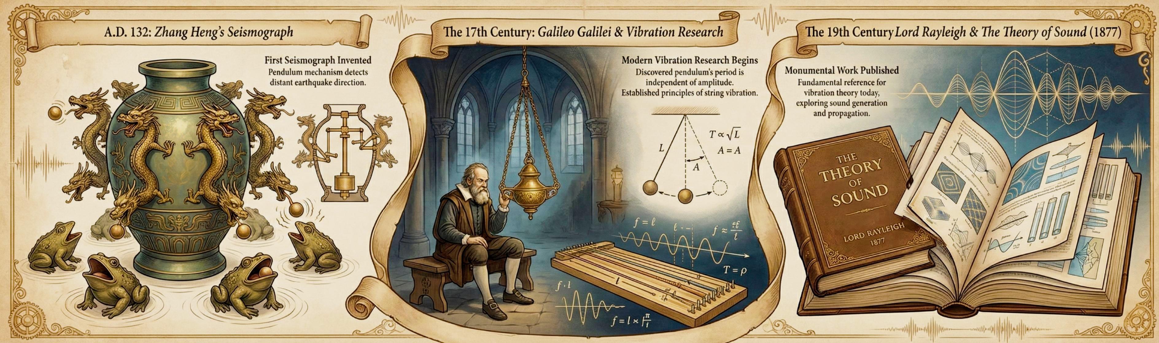
• A.D. 132: The Chinese astronomer Zhang Heng invented the world’s first seismograph. Shaped like a wine jar with dragons and toads, it used a pendulum mechanism to detect the direction of distant earthquakes.
• The 17th Century: Modern vibration research truly began with Galileo Galilei. While observing a swinging lamp in a church in Pisa, Galileo discovered that the period of a pendulum is independent of its amplitude. He also laid the groundwork for understanding the relationship between frequency, length, tension, and density in vibrating strings.
• The 19th Century: Lord Rayleigh published his monumental work, The Theory of Sound, in 1877. This work remains a fundamental reference for vibration theory today.

Why Study Vibration?

Vibration is a double-edged sword in engineering.

• The Destructive Side: Vibration can cause structural failure, noise, and wear. The collapse of the Tacoma Narrows Bridge is a classic example of wind-induced resonance leading to catastrophe.
• The Beneficial Side: Without vibration, we could not speak or hear, as our vocal cords and eardrums rely on oscillatory motion. Industrial applications include vibration screens, conveyors, and hoppers.

As engineers, our goal is simple: to control vibration. We must suppress it when it causes damage and encourage it when it serves a purpose.

The Anatomy of a Vibrating System

Fundamentally, vibration is any motion that repeats itself after an interval of time. A vibratory system consists of three elementary parts:

1. Spring (Stiffness): A means for storing potential energy.
2. Mass (Inertia): A means for storing kinetic energy.
3. Damper: A means by which energy is gradually lost (dissipated).

The classic Single-Degree-of-Freedom (SDOF) model connects these three elements:

Degrees of Freedom (DOF)

One of the most critical concepts in analysis is the “Degree of Freedom.” This is defined as the minimum number of independent coordinates required to determine the position of all parts of a system at any instant.

The Engineering Workflow: Modeling

Real-world systems—like a motorcycle or a skyscraper—are incredibly complex. To analyze them, we must create a mathematical model. Rao outlines a four-step standard procedure for vibration analysis:

1. Mathematical Modeling: The physical system is approximated by using a set of rigid masses, massless springs, and dampers. For example, a motorcycle rider can be modeled as a mass supported by a spring (the seat) and a damper (the body’s natural damping).
2. Derivation of Governing Equations: We use principles like Newton’s second law or the conservation of energy to write the differential equations that describe the motion.
3. Solution of Equations: We solve these differential equations to find the displacement, velocity, and acceleration of the system.
4. Interpretation: Finally, the mathematical results are converted back into physical insights to determine if the design is safe.

Essential Modeling Elements

Springs

Linear springs follow Hooke’s Law: $F = kx$, where $k$ is the spring constant (stiffness).

Dampers

While energy can be lost through friction or air resistance, we often model damping as Viscous Damping. In this model, the damping force is proportional to velocity: $F = cv$, where $c$ is the damping constant. This model is preferred because it leads to linear equations of motion that are easier to solve.

Julia in Action: Visualizing Harmonic Motion

A key feature of modern vibration analysis is the integration of computational tools. Let’s visualize the simplest form of vibration: Simple Harmonic Motion.

The displacement $x$ can be described as $x = A \sin(\omega t)$, where $A$ is the amplitude and $\omega$ is the circular frequency. Here is a Julia script to visualize this:

 1
 2
 3
 4
 5
 6
 7
 8
 9
10
11
12
13
14
15
16
17
18
19
20
21
22
23
24
25
26
27
28
29
30
31

using Plots

# Simple Harmonic Motion Parameters
A = 5.0          # Amplitude (m)
ω = 2.0          # Circular frequency (rad/s)
T = 2π / ω       # Period (s)

# Time vector (3 complete periods)
t = range(0, 3T, length=500)

# Displacement equation: x(t) = A sin(ωt)
x = @. A * sin(ω * t)

# Create plot with professional styling
plot(t, x,
    linewidth = 2,
    color = :royalblue,
    label = "x(t) = A sin(ωt)",
    xlabel = "Time t (s)",
    ylabel = "Displacement x (m)",
    title = "Simple Harmonic Motion",
    legend = :topright,
    grid = true,
    size = (800, 450),
    dpi = 150
)

# Add amplitude annotations
hline!([A, -A], linestyle=:dash, color=:gray, alpha=0.5, label="±A")

savefig("harmonic_motion.png")

Running this code produces a clear visualization showing the sinusoidal oscillation pattern characteristic of undamped free vibration.

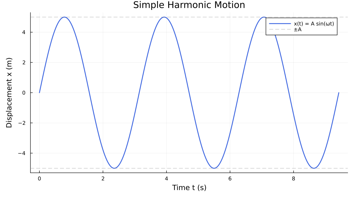
This simple oscillation is the foundation upon which complex vibration theories are built.

What’s Next?

Now that we have defined our system elements, what happens when we pull the mass and let go? In the next post, “Free Vibration of Single-Degree-of-Freedom Systems,” we will derive the equation of motion, calculate natural frequencies, and see exactly how damping brings a vibrating system to rest.

References

Rao, S. S. (2018). Mechanical Vibrations (6th ed.). Pearson.