Mastering the pocket algorithm for non-separable data, understanding parameters vs hyperparameters, and the complete ML training workflow.
Learning Objectives
After reading this post, you will be able to:
Implement the pocket algorithm for non-separable data
Distinguish between parameters and hyperparameters
Explain the train/validation/test split strategy
Perform K-fold cross-validation
Theory
This article covers three key topics: handling non-separable data with the pocket algorithm, understanding the difference between parameters and hyperparameters, and the complete training workflow.
The Problem with Basic Perceptron
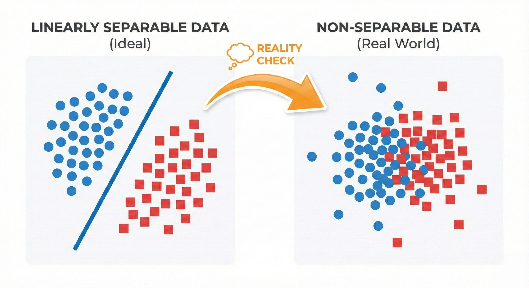
In last post, the perceptron was shown to converge only for linearly separable data. But real-world data often contains:
Noise: Measurement errors or mislabeled samples
Overlapping classes: Genuine class overlap
Comparison diagram: Linearly Separable vs. Non-Separable Data (Real World)
For such data, the basic perceptron will never converge — it keeps oscillating.
The Pocket Algorithm
The pocket algorithm is a simple fix: keep the best weights “in your pocket” while the perceptron keeps updating.
graph LR
A[Initialize\n w, b] --> B[Initialize\n best_w = w,\n best_b = b]
B --> C[Find\n misclassified\n point]
C --> D[Update w, b]
D --> E{New accuracy\n >\n best?}
E -->|Yes| F[Put new weights\n in pocket]
E -->|No| G[Keep pocket\n unchanged]
F --> H{Max iterations?}
G --> H
H -->|No| C
H -->|Yes| I[Return\n pocket weights]
Key insight: Even if the perceptron ends in a bad state, the algorithm returns the best weights ever seen.
Parameters vs Hyperparameters
With the pocket algorithm in hand, the next question is: what values should be used for learning_rate and max_iter? This leads to the distinction between parameters and hyperparameters.
Type
Description
Examples
How to Set
Parameters
Learned from data
Weights $w$, bias $b$
Training algorithm
Hyperparameters
Set before training
Learning rate, max iterations
Cross-validation
💡 Parameters are the model’s “knowledge”; hyperparameters are the model’s “settings.”
The Complete ML Workflow
To properly tune hyperparameters without cheating, data needs to be split strategically. This is the complete ML workflow.
graph LR
A[All Data] --> B[Training Set 60%]
A --> C[Validation Set 20%]
A --> D[Test Set 20%]
B --> E[Train Models]
E --> F[Evaluate on\n Validation]
F --> G{Select\n Best Model}
G --> H[Final Evaluation\n on Test]
style B fill:#c8e6c9
style C fill:#fff9c4
style D fill:#ffcdd2
Dataset
Purpose
When to Use
Training
Learn parameters
During training
Validation
Tune hyperparameters
Model selection
Test
Final evaluation
Only once at the end
⚠️ Never use test data during model development! It must remain “unseen” for honest evaluation.
K-Fold Cross-Validation
What if the dataset is too small for a separate validation set? K-fold cross-validation provides a solution by reusing data more efficiently.
When data is limited, a large validation set may not be affordable. K-fold cross-validation solves this:
graph LR
subgraph "5-Fold Cross-Validation"
F1["Fold 1: Val | Train | Train | Train | Train"]
F2["Fold 2: Train | Val | Train | Train | Train"]
F3["Fold 3: Train | Train | Val | Train | Train"]
F4["Fold 4: Train | Train | Train | Val | Train"]
F5["Fold 5: Train | Train | Train | Train | Val"]
end
F1 --> A[Score 1]
F2 --> B[Score 2]
F3 --> C[Score 3]
F4 --> D[Score 4]
F5 --> E[Score 5]
A --> AVG[Average Score]
B --> AVG
C --> AVG
D --> AVG
E --> AVG
Process:
Split data into K equal parts (folds)
For each fold, use it as validation, train on the rest
importnumpyasnpclassPocketPerceptron:def__init__(self,learning_rate=1.0,max_iter=1000):self.lr=learning_rateself.max_iter=max_iterself.w=Noneself.b=Nonedef_accuracy(self,X,y):predictions=np.sign(np.dot(X,self.w)+self.b)returnnp.mean(predictions==y)deffit(self,X,y):n_samples,n_features=X.shape# Initialize weightsself.w=np.zeros(n_features)self.b=0# Pocket: store best weightsbest_w=self.w.copy()best_b=self.bbest_accuracy=self._accuracy(X,y)foriterationinrange(self.max_iter):# Find a misclassified pointforxi,yiinzip(X,y):ifyi*(np.dot(self.w,xi)+self.b)<=0:# Update weightsself.w+=self.lr*yi*xiself.b+=self.lr*yi# Check if this is bettercurrent_acc=self._accuracy(X,y)ifcurrent_acc>best_accuracy:best_accuracy=current_accbest_w=self.w.copy()best_b=self.bbreakelse:# No misclassifications, we're donebreak# Return the pocket (best) weightsself.w=best_wself.b=best_breturnselfdefpredict(self,X):returnnp.sign(np.dot(X,self.w)+self.b)defscore(self,X,y):returnnp.mean(self.predict(X)==y)
fromsklearn.model_selectionimporttrain_test_split# First split: separate test setX_temp,X_test,y_temp,y_test=train_test_split(X,y,test_size=0.2,random_state=42)# Second split: training and validationX_train,X_val,y_train,y_val=train_test_split(X_temp,y_temp,test_size=0.25,random_state=42# 0.25 * 0.8 = 0.2)print(f"Training set: {len(X_train)} samples ({len(X_train)/len(X):.0%})")print(f"Validation set: {len(X_val)} samples ({len(X_val)/len(X):.0%})")print(f"Test set: {len(X_test)} samples ({len(X_test)/len(X):.0%})")
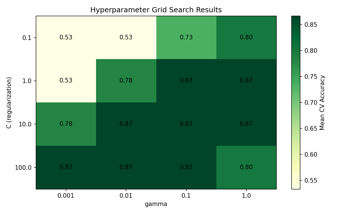
fromsklearn.model_selectionimportGridSearchCVfromsklearn.svmimportSVC# Define hyperparameter gridparam_grid={'C':[0.1,1,10,100],# Regularization strength'gamma':[1,0.1,0.01,0.001]# Kernel coefficient}# Grid search with cross-validationgrid_search=GridSearchCV(SVC(kernel='rbf',random_state=42),param_grid,cv=5,scoring='accuracy')grid_search.fit(X_train,y_train)print(f"Best hyperparameters: {grid_search.best_params_}")print(f"Best CV score: {grid_search.best_score_:.2%}")# Final evaluation on test setbest_model=grid_search.best_estimator_test_accuracy=best_model.score(X_test,y_test)print(f"Test set accuracy: {test_accuracy:.2%}")
Q1: How many folds should I use for cross-validation?
Common choices:
K=5 or K=10: Standard choices, good balance between bias and variance
K=N (Leave-One-Out): Maximum training data, but computationally expensive
Stratified K-Fold: Preserves class proportions in each fold (recommended for imbalanced data)
Q2: What if I have very little data?
Use higher K (more folds) to maximize training data
Consider Leave-One-Out cross-validation
Use data augmentation if applicable
Try simpler models with fewer parameters
Q3: Why not tune hyperparameters on the test set?
If you tune on the test set, you’re essentially “peeking” at it. The reported test accuracy becomes optimistically biased and won’t reflect real-world performance.
Summary
Concept
Key Points
Pocket Algorithm
Keeps best weights during training
Parameters
Learned from data (w, b)
Hyperparameters
Set before training (learning rate, iterations)
Train/Val/Test Split
60/20/20 is typical
K-Fold CV
Average performance across K folds
References
Gallant, S. I. (1990). “Perceptron-based learning algorithms”