ML-02: The Perceptron and Decision Boundaries
Learning Objectives
After reading this post, you will be able to:
- Understand what binary classification means
- Explain the mathematical representation of a decision boundary
- Implement the perceptron algorithm from scratch
- Distinguish between linearly separable and non-separable data
Theory
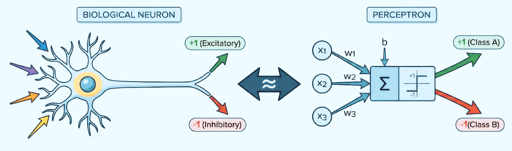
Building on the ML fundamentals from the previous article, this post introduces the perceptron — the simplest neural network and the foundation of deep learning.
Binary Classification Problem
Consider a bank evaluating credit card applications. Based on historical data:
| Applicant | Annual Income | Debt Ratio | Approved? |
|---|---|---|---|
| Alice | $80,000 | 0.2 | ✅ Yes |
| Bob | $30,000 | 0.8 | ❌ No |
| Carol | $60,000 | 0.3 | ✅ Yes |
| Dave | $40,000 | 0.6 | ❌ No |
This is a binary classification problem: we want to classify new applicants into two groups (approved/rejected).
The Decision Boundary
When plotting the data on a 2D plane (income vs. debt ratio), we observe that approved and rejected applicants can be separated by a line:
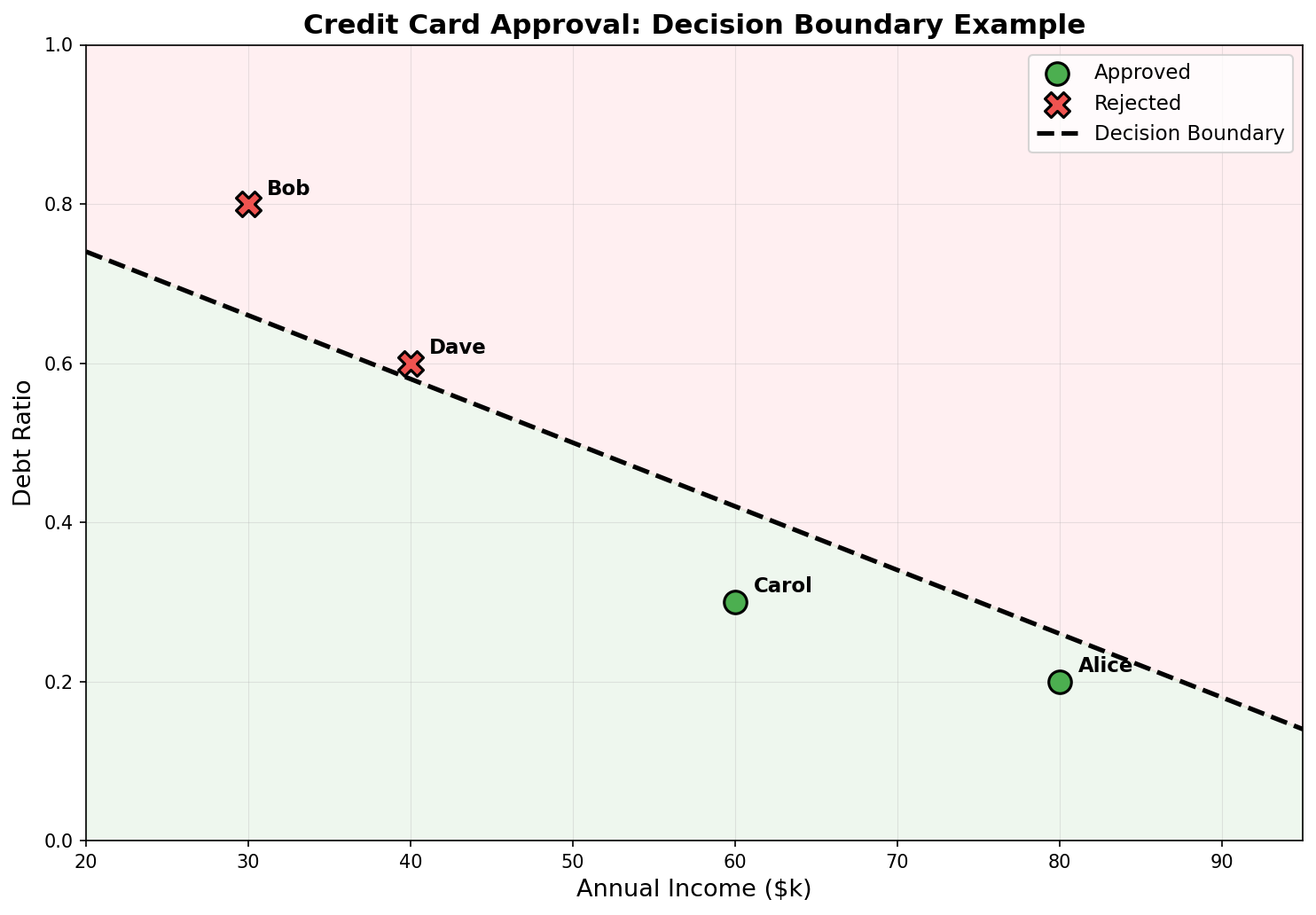
This separating line is called the decision boundary.
Mathematical Formulation
How can this separating line be described mathematically? This is where the decision boundary equation comes in.
A line in 2D can be written as:
$$w_1 x_1 + w_2 x_2 + b = 0$$
Or in vector form:
$$\boldsymbol{w} \cdot \boldsymbol{x} + b = 0$$
Where:
- $\boldsymbol{w} = (w_1, w_2)$ is the weight vector (normal to the line)
- $\boldsymbol{x} = (x_1, x_2)$ is the input features
- $b$ is the bias term
The Perceptron Model
With the mathematical representation in place, the next step is to define how the model makes predictions.
The perceptron classifies a point based on which side of the line it falls:
$$h(\boldsymbol{x}) = \text{sign}(\boldsymbol{w} \cdot \boldsymbol{x} + b)$$
Where the sign function returns:
- $+1$ if $\boldsymbol{w} \cdot \boldsymbol{x} + b > 0$
- $-1$ if $\boldsymbol{w} \cdot \boldsymbol{x} + b < 0$
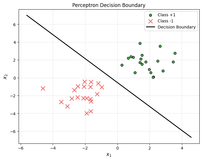
Linear Separability
The perceptron works perfectly when classes can be separated by a line. But what does “separable” really mean?
A dataset is linearly separable if there exists a line (or hyperplane) that perfectly separates the two classes:
| Linearly Separable | Not Linearly Separable |
|---|---|
| A line can separate all points | No line can perfectly separate |
| Perceptron converges | Perceptron may not converge |
The Perceptron Learning Algorithm
The perceptron learns iteratively by examining each training example and adjusting weights when misclassifications occur:
Algorithm:
Intuition: When a point is misclassified, we “push” the decision boundary toward the correct side.
Code Practice
Now let’s implement everything from scratch and see the perceptron in action.
Implementing the Perceptron from Scratch
🐍 Python
| |
Testing on Linearly Separable Data
🐍 Python
| |
Output:
Visualizing the Decision Boundary
🐍 Python
| |
What Happens with Non-Separable Data?
🐍 Python
| |
Output:
| |
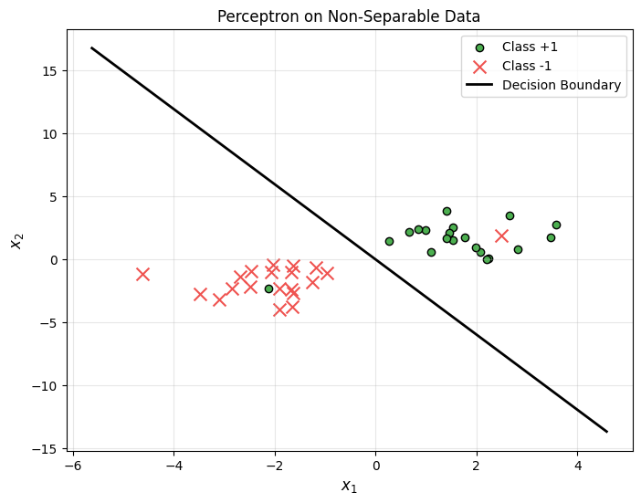
The perceptron still finds a reasonable boundary, but it can’t achieve 100% accuracy on non-separable data.
Using sklearn’s Perceptron
🐍 Python
| |
Output:
| |
Deep Dive
Q1: Why does the perceptron update rule work?
When a point $(x_i, y_i)$ is misclassified, updating $w \leftarrow w + y_i x_i$ moves the decision boundary to correctly classify that point. The dot product $w \cdot x_i$ increases by $y_i |x_i|^2$, pushing the output toward the correct sign.
Q2: What if data isn’t linearly separable?
The basic perceptron will oscillate forever without converging. Solutions include:
- Pocket Algorithm: Keep track of the best weights seen so far
- Soft-margin methods: Allow some misclassifications
Q3: Perceptron vs. Logistic Regression?
| Aspect | Perceptron | Logistic Regression |
|---|---|---|
| Output | Hard decision (+1/-1) | Probability (0-1) |
| Loss Function | Misclassification count | Cross-entropy |
| Non-separable data | May not converge | Always converges |
Summary
| Concept | Key Points |
|---|---|
| Binary Classification | Classifying into two groups |
| Decision Boundary | $\boldsymbol{w} \cdot \boldsymbol{x} + b = 0$ |
| Perceptron | $h(\boldsymbol{x}) = \text{sign}(\boldsymbol{w} \cdot \boldsymbol{x} + b)$ |
| Linear Separability | A line can perfectly separate classes |
| Update Rule | $\boldsymbol{w} \leftarrow \boldsymbol{w} + y_i \boldsymbol{x}_i$ |
References
- Rosenblatt, F. (1958). The Perceptron: A Probabilistic Model for Information Storage and Organization in the Brain . Psychological Review, 65(6), 386–408.
- Perceptron - Wikipedia
- sklearn Perceptron Documentation
- Abu-Mostafa, Y. S., Magdon-Ismail, M., & Lin, H. T. (2012). Learning From Data. AMLBook.