ML-01: Introduction to Machine Learning

Publish on: 2022/04/06 Classify at: CODE/Machine Learning

Words: 1402 Read:≈ 7min

Summary

Understanding what machine learning is through the self-driving car example, mastering the core concepts of training and prediction.

A futuristic self-driving car navigating a city street — Figure 1: Concept art of a self-driving vehicle.

Learning Objectives

After reading this post, you will be able to:

Understand the fundamental difference between machine learning and traditional programming
Know the three conditions where machine learning is applicable
Master the core concepts of “training” and “prediction”
Distinguish between supervised, unsupervised, reinforcement, and deep learning

Theory

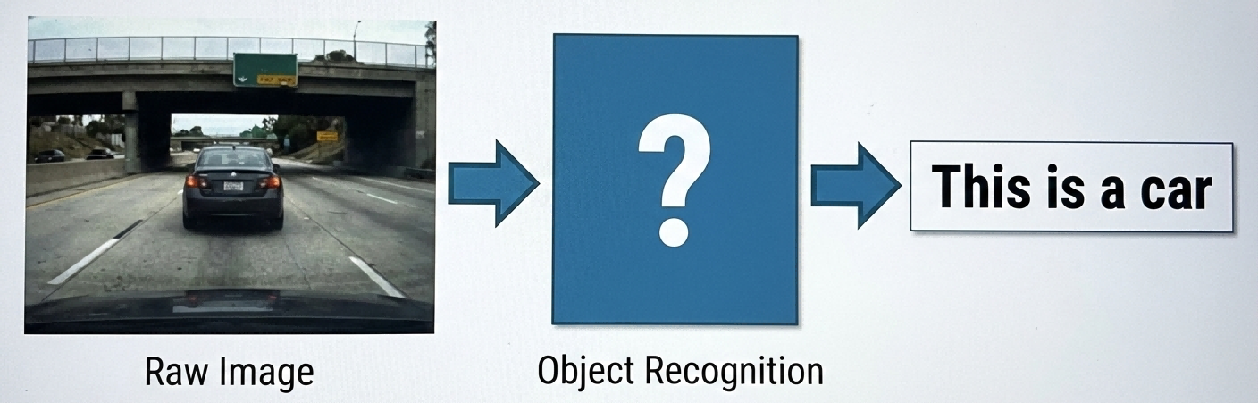
The Self-Driving Car Challenge

Imagine a self-driving car navigating through traffic. It needs to constantly “see” its surroundings and identify pedestrians, vehicles, traffic lights, etc.:

Object recognition challenge: camera feed to unknown process to classification result — **Figure 2:** The object recognition challenge — Camera Feed → [???] → Classification

What goes in [???]? Traditional programming might approach it like this:

1
2
3
4
5
# Traditional programming approach (pseudocode)
def is_car(image):
    if has_four_wheels(image) and has_windows(image) and has_headlights(image):
        return True
    return False

But here’s the problem:

What if half the car is occluded, showing only two wheels?
What about trucks, motorcycles, or exotic vehicles?
Real-world scenarios are too complex to enumerate all rules!

This is where machine learning comes in.

What is Machine Learning?

Machine learning takes a completely different approach:

1
2
3
Thousands of car images + labels → [Learning Algorithm] → Model

New unknown image → [Model] → "This is a car"

Instead of telling the machine “cars have four wheels,” we show it thousands of car images and let it learn on its own what a car is.

Training and Prediction

Machine learning consists of two core steps:

Step	Description	Analogy
Training	Teaching the machine using known data	Student doing practice problems
Prediction	Making judgments on new data	Student taking an exam

💡 Key Question: Why does performing well on practice problems translate to good exam performance? This will be answered in later posts!

When to Use Machine Learning

Not every problem is suitable for machine learning. Three conditions must be met:

Using self-driving as an example:

✅ Pattern exists: All cars share common features
✅ Hard to define: Can’t describe “what is a car” with simple rules
✅ Data available: Internet has countless car images

Types of Machine Learning

Type	Core Idea	Typical Applications
Supervised Learning	Has “teacher” guidance, data with labels	Handwriting recognition, spam filtering
Unsupervised Learning	No labels, discovers patterns	Customer segmentation, recommendations
Reinforcement Learning	Learns through trial and error	Game AI, robotics
Deep Learning	Simulates brain’s neural networks	Image recognition, voice assistants

📚 This series focuses on: Supervised Learning

Supervised Learning Example

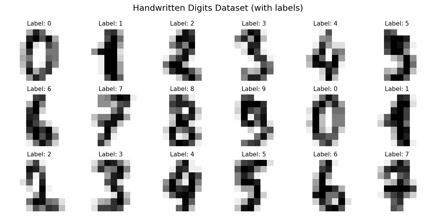
In supervised learning, each training sample has a label — like homework graded by a teacher:

1
2
3
4
5
Image1 + label "cat" 
Image2 + label "dog"
Image3 + label "cat"
...
→ After learning, can recognize new cat/dog images

Code Practice

Environment Setup

🐍 Python

1
2
# Required libraries
# pip install numpy matplotlib scikit-learn

Meet Your First Dataset: Handwritten Digits

Let’s load the classic handwritten digits dataset to see what “labeled data” looks like:

🐍 Python

 1
 2
 3
 4
 5
 6
 7
 8
 9
10
import matplotlib.pyplot as plt
from sklearn import datasets

# Load handwritten digits dataset
digits = datasets.load_digits()

# Basic dataset info
print(f"Dataset size: {len(digits.images)} images")
print(f"Image shape: {digits.images[0].shape}")  # 8x8 pixels
print(f"Label range: {digits.target.min()} ~ {digits.target.max()}")

Output:

1
2
3
Dataset size: 1797 images
Image shape: (8, 8)
Label range: 0 ~ 9

Visualizing Labeled Data

🐍 Python

 1
 2
 3
 4
 5
 6
 7
 8
 9
10
11
12
# Visualize some digits with their labels
fig, axes = plt.subplots(3, 6, figsize=(10, 5))
fig.suptitle('Handwritten Digits Dataset (with labels)', fontsize=14)

for i, ax in enumerate(axes.flat):
    ax.imshow(digits.images[i], cmap='gray_r')
    ax.set_title(f'Label: {digits.target[i]}', fontsize=10)
    ax.axis('off')

plt.tight_layout()
plt.show()
plt.savefig('assets/digits_labeled.png', dpi=150)

MNIST handwritten digits 0-9 with labels — **Figure 3:** Sample handwritten digits from the MNIST dataset

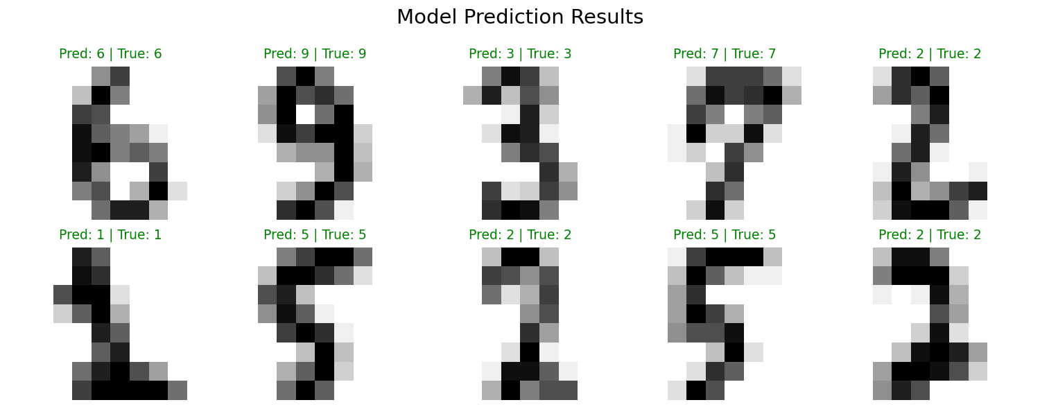
Experience Training and Prediction

Although we haven’t learned specific algorithms yet, let’s experience the complete ML workflow:

🐍 Python

 1
 2
 3
 4
 5
 6
 7
 8
 9
10
11
12
13
14
15
16
17
18
19
20
21
22
23
24
25
26
from sklearn.model_selection import train_test_split
from sklearn.neighbors import KNeighborsClassifier
from sklearn.metrics import accuracy_score

# Prepare data
X = digits.data      # Features: pixel values
y = digits.target    # Labels: 0-9

# Split into training and test sets
X_train, X_test, y_train, y_test = train_test_split(
    X, y, test_size=0.2, random_state=42
)

print(f"Training set size: {len(X_train)}")
print(f"Test set size: {len(X_test)}")

# Train model (using K-Nearest Neighbors, will cover later)
model = KNeighborsClassifier(n_neighbors=3)
model.fit(X_train, y_train)  # This is "training"

# Predict
y_pred = model.predict(X_test)  # This is "prediction"

# Evaluate accuracy
accuracy = accuracy_score(y_test, y_pred)
print(f"\nModel accuracy on test set: {accuracy:.2%}")

Output:

1
2
3
4
Training set size: 1437
Test set size: 360

Model accuracy on test set: 98.33%

Visualizing Predictions

🐍 Python

 1
 2
 3
 4
 5
 6
 7
 8
 9
10
11
12
13
14
# Show some prediction results
fig, axes = plt.subplots(2, 5, figsize=(10, 4))
fig.suptitle('Model Prediction Results', fontsize=14)

for i, ax in enumerate(axes.flat):
    ax.imshow(X_test[i].reshape(8, 8), cmap='gray_r')
    color = 'green' if y_pred[i] == y_test[i] else 'red'
    ax.set_title(f'Pred: {y_pred[i]} | True: {y_test[i]}', 
                 fontsize=9, color=color)
    ax.axis('off')

plt.tight_layout()
plt.show()
plt.savefig('assets/predictions.png', dpi=150)

Try Your Own Handwriting

Now comes the fun part — test the model with your own handwritten digit!

🐍 Python

 1
 2
 3
 4
 5
 6
 7
 8
 9
10
11
12
13
14
15
16
17
18
19
20
21
22
23
24
25
26
27
28
29
30
31
32
33
34
35
36
37
38
39
40
41
42
43
44
45
46
47
48
49
50
51
52
53
54
55
56
57
58
59
60
61
62
63
64
65
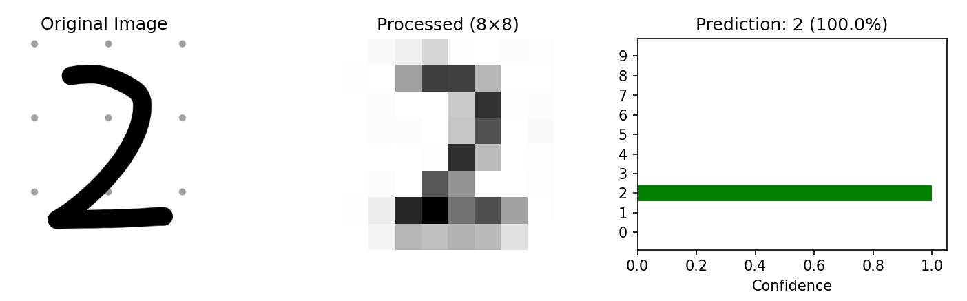
from PIL import Image
import numpy as np
import matplotlib.pyplot as plt
from sklearn.datasets import load_digits
from sklearn.neighbors import KNeighborsClassifier

# Train the model (same as before)
digits = load_digits()
X, y = digits.data, digits.target
clf = KNeighborsClassifier(n_neighbors=3)
clf.fit(X, y)

def predict_custom_digit(image_path, visualize=True):
    """
    Load a custom handwritten digit image and predict its value.
    Image should be a white digit on black background, any size.
    """
    # Load original image
    img_original = Image.open(image_path).convert('L')
    
    # Resize to 8x8
    img_resized = img_original.resize((8, 8), Image.Resampling.LANCZOS)
    
    # Convert to array and normalize (sklearn digits are 0-16 scale)
    img_array = np.array(img_resized)
    img_processed = 16 - (img_array / 255.0 * 16)  # Invert colors
    img_flat = img_processed.flatten().reshape(1, -1)
    
    # Predict
    prediction = clf.predict(img_flat)[0]
    probabilities = clf.predict_proba(img_flat)[0]
    confidence = probabilities[prediction] * 100
    
    # Visualization
    if visualize:
        fig, axes = plt.subplots(1, 3, figsize=(10, 3))
        
        # Original image
        axes[0].imshow(img_original, cmap='gray')
        axes[0].set_title('Original Image')
        axes[0].axis('off')
        
        # Processed 8x8 image
        axes[1].imshow(img_processed, cmap='gray_r')
        axes[1].set_title('Processed (8×8)')
        axes[1].axis('off')
        
        # Prediction confidence bar
        colors = ['green' if i == prediction else 'lightgray' for i in range(10)]
        axes[2].barh(range(10), probabilities, color=colors)
        axes[2].set_yticks(range(10))
        axes[2].set_xlabel('Confidence')
        axes[2].set_title(f'Prediction: {prediction} ({confidence:.1f}%)')
        
        plt.tight_layout()
        plt.savefig('assets/custom_prediction.png', dpi=150)
        plt.show()
    
    print(f"Predicted digit: {prediction}")
    print(f"Confidence: {confidence:.1f}%")
    
    return prediction

# Usage example:
predict_custom_digit('my_digit.png')

Custom handwriting prediction visualization showing original image, processed 8x8 grid, and confidence scores — **Figure 5:** Custom digit prediction — Original image, preprocessed input, and model confidence

💡 Tips for best results:
Draw a white digit on black background
Center the digit in the image
Use a thick brush/pen stroke
Save as PNG format

Deep Dive

Q1: Why does learning from training data work on new data?

This is the core question of machine learning! Simply put, we assume training and test data come from the same distribution.

Q2: Deep learning is so powerful — why learn traditional ML?

Deep learning requires massive datasets; traditional methods may work better on small data
Deep learning needs powerful hardware (GPUs); traditional methods are lighter
Traditional methods offer better interpretability — they can tell you “why” a prediction was made

Q3: How do I choose which ML method to use?

Summary

Core Concept	Key Points
Machine Learning	Machines learn from data instead of explicit programming
Training	Teaching the model with labeled data
Prediction	Making judgments on new data
Applicability	Pattern exists + Hard to define + Data available
Supervised Learning	The focus of this series; data has labels

References

scikit-learn Digits Dataset Documentation
“Pattern Recognition and Machine Learning” by Christopher Bishop - Chapter 1
3Blue1Brown: Neural Networks Introduction