Introduction

When data is represented as a function of time or space, the Fourier transform decomposes the data into frequency components. Fourier transforms can be used to analyze variations in data, such as natural events over a time period.

Astronomers have tabulated the quantity and size of sunspots for nearly 300 years using the Zurich relative sunspot number. This article will use the Julia language to perform FFT analysis on sunspot data from approximately 1749 to 2024, revealing the periodic patterns of solar activity.

Data Source

The sunspot data used in this analysis comes from SILSO (Sunspot Index and Long-term Solar Observations) , which is the World Data Center for sunspot index maintained by the Royal Observatory of Belgium.

• Data File: SN_m_tot_V2.0.csv - Monthly mean total sunspot number
• Time Coverage: 1749 to present (275+ years of continuous observations)
• Data Format: Year, Month, Decimal Year, Sunspot Number, Standard Deviation, Observations, Marker

SILSO provides the most authoritative and complete record of solar activity, serving as the reference dataset for solar cycle research worldwide.

Loading Data

First, we need to load the sunspot data. The data comes from the SILSO (Sunspot Index and Long-term Solar Observations) database.

 1
 2
 3
 4
 5
 6
 7
 8
 9
10
11
12
13
14

using FFTW          # FFT library
using Plots         # Plotting library
using DelimitedFiles # For reading data files
using Statistics    # Statistical functions

# Read SILSO format monthly data
data = readdlm("SN_m_tot_V2.0.csv", ';')

# Extract year and relative sunspot number
years = Float64.(data[:, 3])        # Decimal year
sunspots = Float64.(data[:, 4])     # Relative sunspot number

println("Data points: $(length(years))")
println("Time range: $(minimum(years)) - $(maximum(years))")

Plotting Sunspot Numbers vs Year

First, let’s visualize the entire time series to observe nearly 300 years of sunspot activity history:

1
2
3
4
5
6
7
8

plot(years, sunspots,
    xlabel = "Year",
    ylabel = "Zurich Relative Sunspot Number",
    title = "Sunspot Data",
    linewidth = 0.8,
    color = :blue,
    legend = false,
    framestyle = :box)

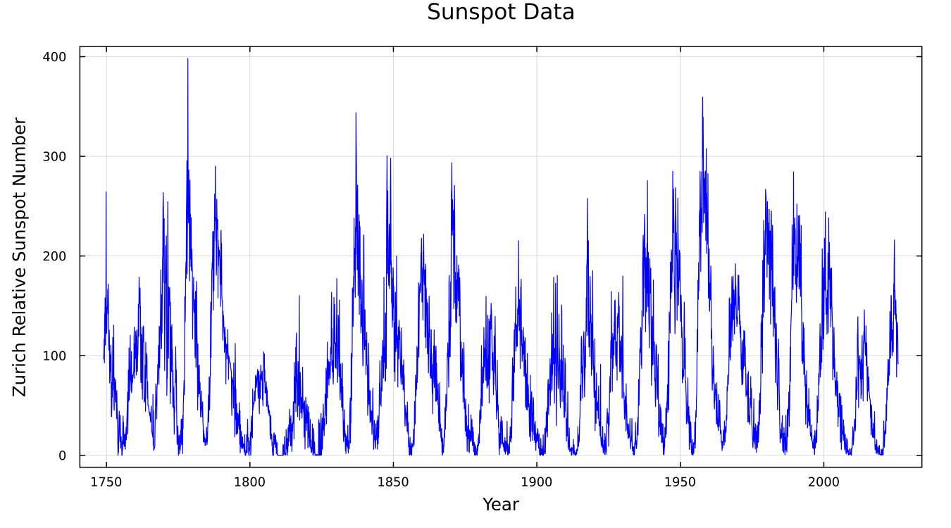
From the plot, we can clearly see that sunspot numbers exhibit regular fluctuations, suggesting some kind of periodicity.

Local Data Observation

To see the periodic characteristics of sunspot activity in more detail, we plot the first 50 months of data:

1
2
3
4
5
6
7
8
9

plot(years[1:50], sunspots[1:50],
    xlabel = "Year",
    ylabel = "Zurich Relative Sunspot Number",
    title = "First 50 Months of Sunspot Data",
    linewidth = 1.5,
    color = :blue,
    marker = :circle,
    markersize = 3,
    framestyle = :box)

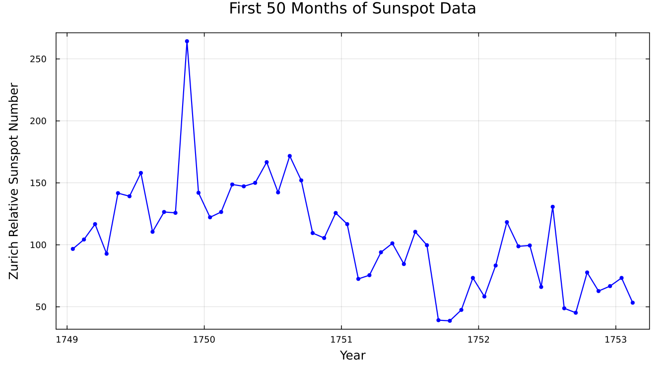
When zoomed in, we can see the monthly data fluctuations, with these short-term variations superimposed on the long-term cycle.

Fourier Transform

The fft function can be used to get the Fourier transform of the sunspot data. Remove the first element of the output (DC component), and plot the distribution of Fourier coefficients on the complex plane, which shows the complex Fourier coefficients as a mirror image about the real axis:

 1
 2
 3
 4
 5
 6
 7
 8
 9
10
11
12
13
14
15

# Compute FFT
y = fft(sunspots)

# Remove DC component (first element, representing signal mean)
y_no_dc = y[2:end]

# Plot Fourier coefficients on complex plane
scatter(real.(y_no_dc), imag.(y_no_dc),
    xlabel = "Real(Y)",
    ylabel = "Imag(Y)",
    title = "Fourier Coefficients",
    markersize = 2,
    color = :red,
    alpha = 0.6,
    framestyle = :box)

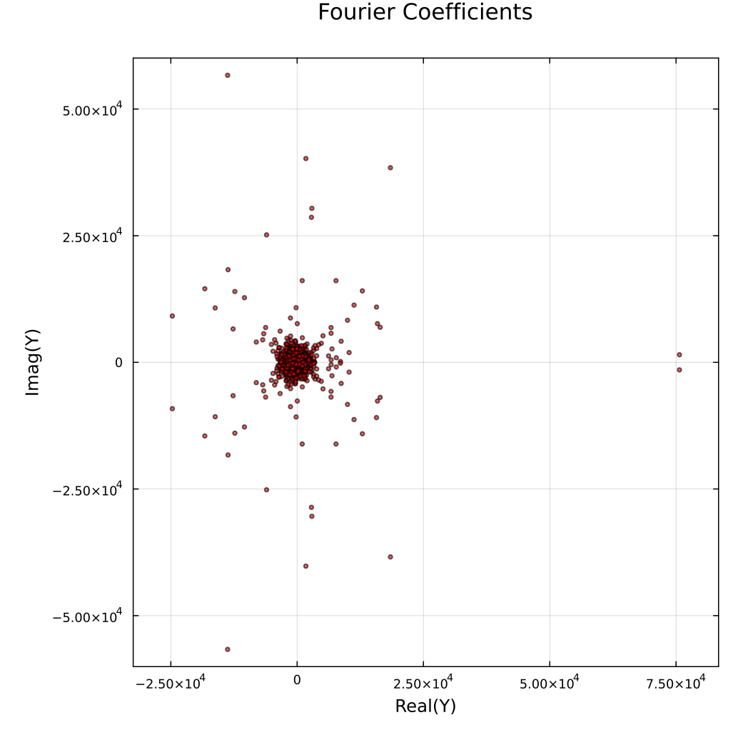
The distribution of Fourier coefficients on the complex plane shows symmetry, which is an inherent property of FFT for real signals.

Power Spectrum

Individual Fourier coefficients are difficult to interpret. We plot the spectrum as a function of frequency, measured in cycles per year:

 1
 2
 3
 4
 5
 6
 7
 8
 9
10
11
12
13
14
15

n = length(y_no_dc)

# Calculate power spectrum = |FFT coefficients|²
power = abs.(y_no_dc[1:n÷2]).^2

# Calculate frequency axis (cycles/year)
maxfreq = 0.5  # Nyquist frequency
freq = (1:n÷2) ./ (n÷2) .* maxfreq .* 12  # Convert to cycles/year

plot(freq, power,
    xlabel = "Frequency (Cycles/Year)",
    ylabel = "Power",
    title = "Sunspot Power Spectrum",
    xlims = (0, 1.0),
    framestyle = :box)

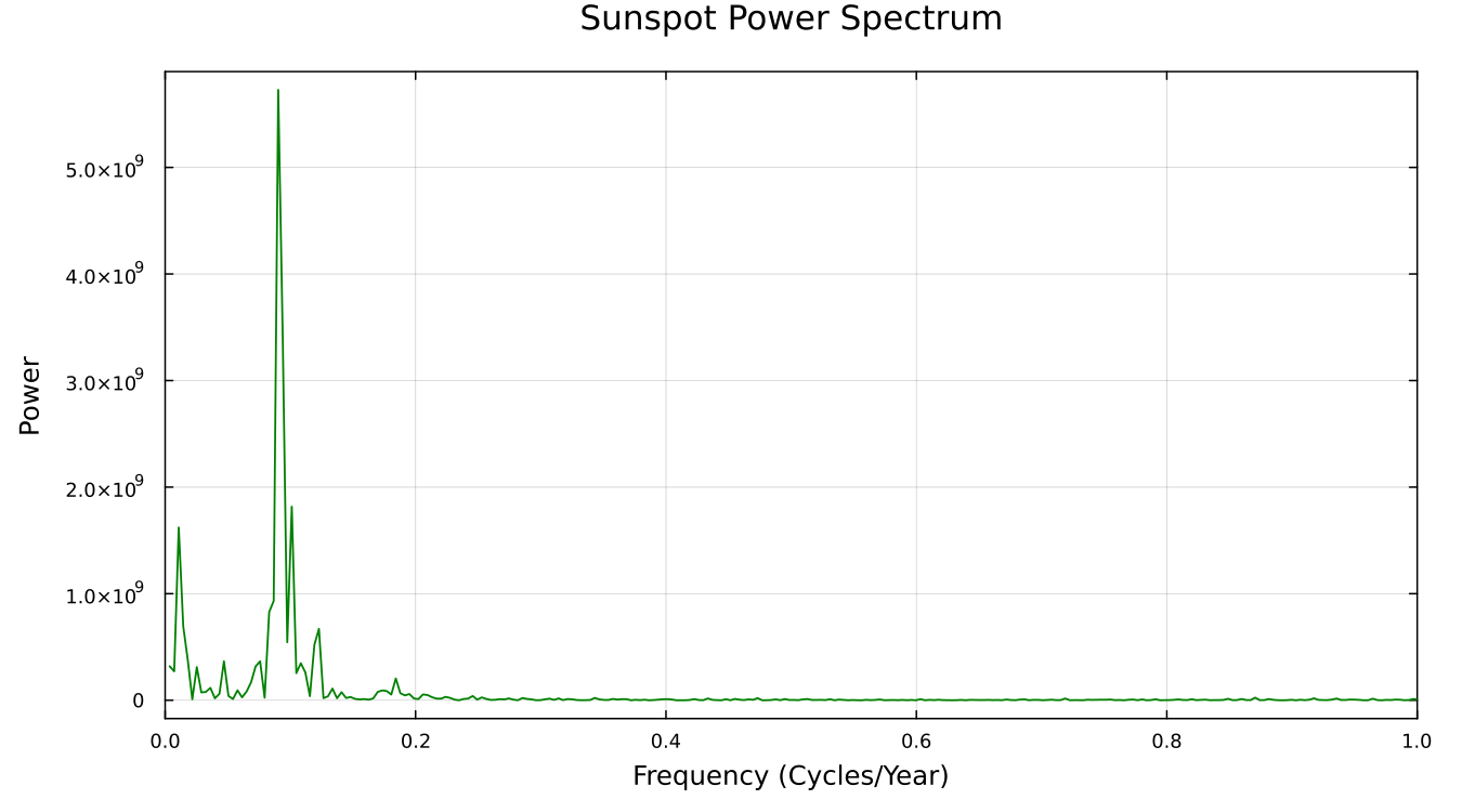
We can see that the maximum frequency of sunspot activity is less than once per year. There is a clear peak in the low frequency region.

Period Domain Analysis

Since the main period is greater than 1 year, plotting as a function of period is more intuitive:

1
2
3
4
5
6
7
8
9

# Calculate period = 1/frequency
period = 1.0 ./ freq

plot(period, power,
    xlabel = "Period (Years/Cycle)",
    ylabel = "Power",
    title = "Sunspot Activity Period",
    xlims = (0, 50),
    framestyle = :box)

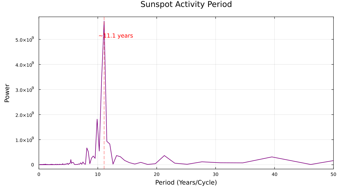
Analysis Conclusions

From the period spectrum, we can clearly see:

Sunspot activity peaks approximately every 11 years.

This is the famous Schwabe Cycle, first discovered by German pharmacist and amateur astronomer Samuel Heinrich Schwabe in 1843.

Importance of the Sunspot Cycle

1. Space Weather Forecasting: Solar flares and coronal mass ejections are more frequent during sunspot activity peaks
2. Satellite Communications: Solar activity affects the ionosphere, which in turn affects radio communications
3. Climate Research: Solar activity cycles may have some correlation with Earth’s climate
4. Power Grid Protection: Intense solar activity can cause geomagnetic storms, affecting power transmission systems

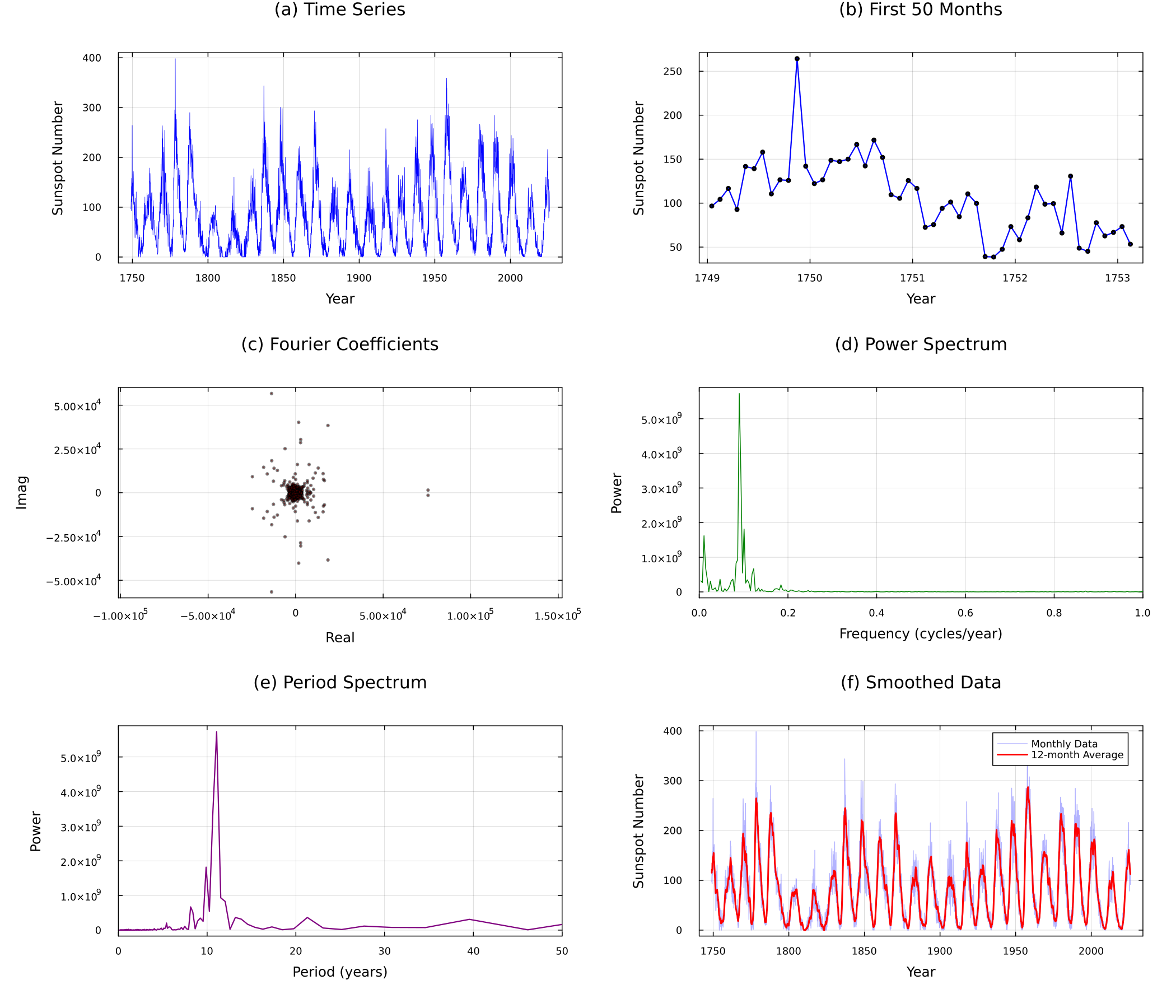
Comprehensive Analysis Plot

Finally, we summarize all analysis results into one figure:

Summary

Through Julia’s FFT analysis, we successfully:

1. Loaded and visualized nearly 300 years of historical sunspot data
2. Used the Fast Fourier Transform to convert time domain signals to frequency domain
3. Discovered the ~11-year dominant period through power spectrum analysis
4. Verified the famous Schwabe solar cycle

This example demonstrates the power of FFT in scientific data analysis - with just a few lines of code, we can extract meaningful periodic information from seemingly chaotic time series data.

Data source: SILSO World Data Center