Simulating Smart Temperature Control in Electric Kettles with COMSOL: A Multiphysics Modeling Guide
Introduction
Picture this: you’ve just boiled water for tea, but get distracted by a phone call. Ten minutes later, your electric kettle has kept the water perfectly warm—not too hot, not too cold. This seemingly simple “keep warm” function actually involves a sophisticated dance of physics.
Natural convection, often overlooked in everyday life, plays a starring role here. The same phenomenon that drives ocean currents and weather patterns also governs the gentle circulation of water in your kettle. From chemical reactors to fermentation vessels, understanding these convective flows is key to optimizing thermal systems.
What makes this problem particularly interesting is the coupling of multiple physical processes:
- Heat Conduction: Energy flowing through the glass walls and steel heating plate
- Natural Convection: Gravity-driven water circulation caused by temperature differences
- Heat Loss: Energy escaping from the kettle surface to the surrounding air
- Species Transport: How dissolved substances get mixed by the swirling water
- Thermostat Control: The on-off switching logic that maintains your target temperature
In this article, we build a 2D axisymmetric COMSOL model to simulate these phenomena, drawing inspiration from the classic “Free Convection in a Water Glass” example in the COMSOL Application Gallery.
mindmap
  root((Electric Kettle Simulation))
    Physics
      Heat Conduction
      Natural Convection
      Species Transport
      Heat Loss
    Control
      Thermostat Logic
      Hysteresis Control
    COMSOL Setup
      Laminar Flow
      Heat Transfer
      Transport of Species
      Events Interface
    Results
      Temperature Field
      Flow Patterns
      Species Mixing
      Energy Balance
Physical Problem Description
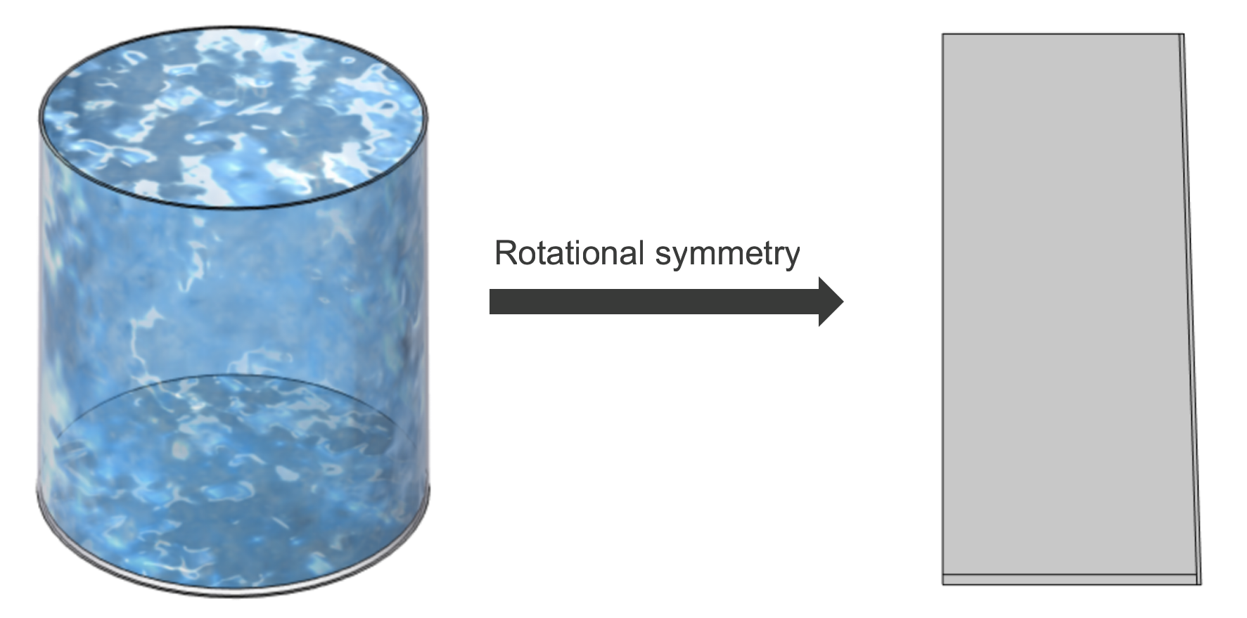
Geometric Model
To keep the simulation tractable, we simplify the electric kettle as an axisymmetric frustum-shaped container. Thanks to rotational symmetry, we can capture all the essential physics in a 2D model—dramatically reducing computational cost without sacrificing accuracy.
Geometric Parameters:
| Parameter | Value | Description |
|---|---|---|
| R_top | 7 cm | Top radius of kettle |
| R_bottom | 7.5 cm | Bottom radius of kettle |
| H_kettle | 16 cm | Kettle height |
| T_wall | 1.3 mm | Glass wall thickness |
| T_bottom | 3 mm | Steel bottom thickness |
Physical Processes
Heat Conduction
In the solid regions—the glass walls and steel heating plate—heat travels by conduction, following Fourier’s law:
$$q = -k \nabla T$$
Here, $k$ is the thermal conductivity and $T$ is temperature. For the glass wall, we use the thermal properties of silica glass.
Natural Convection (Boussinesq Approximation)
The magic happens in the water. When the bottom heats up, warmer water becomes less dense and rises, while cooler water near the walls sinks down to take its place. This creates a continuous circulation pattern—classic Rayleigh-Bénard convection.
We model this density variation using the Boussinesq approximation:
$$\rho = \rho_{ref} [1 - \alpha_p (T - T_{ref})]$$
where $\alpha_p$ is the thermal expansion coefficient. The resulting buoyancy-driven flow forms characteristic recirculation cells that efficiently mix and heat the water.
Species Transport
Beyond heat, we also track how dissolved species (think minerals or tea extract) get distributed. The concentration evolves through:
- Convective transport: Species carried along by the flowing water
- Diffusion: Molecules spreading from high to low concentration
This coupling beautifully demonstrates how natural convection accelerates mixing far beyond what diffusion alone could achieve.
Thermostat Control Logic
The thermostat employs a hysteresis control strategy to prevent rapid on-off cycling:
The heating plate temperature switches according to state:
- Heating state: T_heater = 80°C
- Off state: T_heater = 25°C (room temperature)
COMSOL Model Setup
Physics Interfaces
Translating our physical understanding into COMSOL requires four key physics interfaces:
| Interface | Identifier | Purpose |
|---|---|---|
| Laminar Flow | spf | Simulate buoyancy-driven water flow |
| Heat Transfer in Fluids | ht | Simulate heat conduction and convection |
| Transport of Diluted Species | tds | Track species concentration distribution |
| Events | ev | Implement thermostat switching logic |
Multiphysics Coupling
Non-Isothermal Flow: This is where the magic happens. By coupling Laminar Flow with Heat Transfer and enabling the Boussinesq approximation, temperature differences directly drive fluid motion.
Species Transport Coupling: The diluted species interface “rides along” with the velocity field, letting us track how substances get stirred by the convective currents.
Material Properties
Water (Temperature-Dependent Properties)
Water’s physical properties vary significantly with temperature—a critical factor for accurate natural convection modeling:
| Temperature | Density ρ (kg/m³) | Viscosity η (mPa·s) | Thermal Conductivity k (W/m·K) | Heat Capacity Cp (J/kg·K) |
|---|---|---|---|---|
| 20°C | 998.2 | 1.002 | 0.598 | 4182 |
| 50°C | 988.1 | 0.547 | 0.644 | 4181 |
| 80°C | 971.8 | 0.355 | 0.670 | 4198 |
Note: The model uses piecewise polynomial fits of these properties. See the Appendix for the complete MATLAB implementation.
Solid Materials
| Material | Thermal Conductivity | Density | Heat Capacity |
|---|---|---|---|
| Silicate Glass | 1.38 W/(m·K) | 2203 kg/m³ | 703 J/(kg·K) |
| Structural Steel | 44.5 W/(m·K) | 7850 kg/m³ | 475 J/(kg·K) |
Boundary Conditions
The boundary conditions are carefully chosen to represent realistic physical scenarios:
| Boundary | Condition Type | Setting |
|---|---|---|
| Heating plate bottom | Temperature boundary | T = T_heater_off + (T_heater_on - T_heater_off) × HeaterState |
| Kettle sidewall exterior | Natural convection | External natural convection with heat transfer coefficient, T_amb = 25°C |
| Water surface | Convective heat flux | h = 2 W/(m²·K), driven by temperature difference: $q = h(T_{ext} - T)$ |
| Water surface | Slip wall | No tangential stress (free surface approximation) |
| Glass-water interface | No-slip wall | Zero velocity at solid boundaries |
| Axis of symmetry | Axial symmetry | Symmetry condition for all fields |
Note: Because of the relatively low values of heat transfer film coefficients at the top and side surfaces, a significant portion of heat may be conducted through the bottom boundary when the heater is off. The Heat Transfer Module provides a library of heat transfer coefficient functions that can be utilized for more accurate modeling.
Event Control (Thermostat)
The COMSOL Events interface implements the temperature control logic:
| |
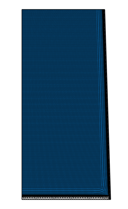
Mesh Configuration
Structured mesh with refinement in boundary layer regions to capture the thin thermal and velocity boundary layers near walls:
- Water domain: Mapped mesh, maximum element size 1 mm
- Boundary layers: 6 boundary layer mesh layers
- Solid regions: Free triangular mesh
Solver Settings
Time Stepping
- Time range: 0 to 3 minutes
- Time step: 3 seconds
- Relative tolerance: 1×10⁻³
- Absolute tolerance: 2.5×10⁻⁵
Nonlinear Solver
Fully Coupled solver with direct solver (PARDISO). This approach handles the strong coupling between momentum, energy, and species transport equations effectively.
Results and Discussion
Let’s see what our simulation reveals!
Temperature Field Evolution

The simulation starts with water at a uniform 49°C—just below the thermostat’s lower threshold. As soon as the heater kicks in, we see the physics spring to life.
The temperature distribution shows characteristic features of Rayleigh-Bénard convection:
- Hot thermal plumes rising from the heating plate
- Cold water descending along the cooler side walls
- Gradual homogenization due to convective mixing
Natural Convection Flow Field
The streamlines tell a beautiful story of organized chaos. Buoyancy drives clear recirculation patterns—convection cells that act like tiny heat pumps, efficiently moving energy from the hot bottom to the cooler top.
Notice how:
- Central upward flow of heated water
- Peripheral downward flow of cooled water
- Multiple recirculation cells may form depending on the Rayleigh number
Species Concentration Distribution
Here’s where things get practical. Imagine you’ve dropped a tea bag or dissolved some minerals. The species transport results show how convection dramatically speeds up mixing:
- Initial concentration hotspots quickly spread throughout the kettle
- Convection outpaces diffusion by orders of magnitude
- Concentration contours follow the flow streamlines like tracer particles
Average Temperature Curve
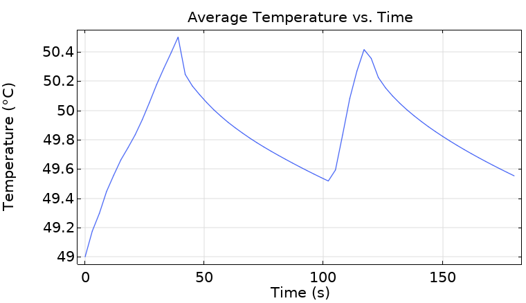
The thermostat does its job beautifully! The average water temperature oscillates between 49.5°C and 50.5°C—exactly as designed. The sawtooth pattern reveals:
- Rapid initial heating when heater is on
- Gradual cooling when heater is off due to heat loss to the environment
- Hysteresis prevents rapid on-off switching
Heat Flux Analysis
| Boundary | Heat Flux Direction | Description |
|---|---|---|
| Heating plate (when on) | Inflow (+Q_in) | Primary heat source |
| Sidewall | Outflow (-Q_wall) | Convective loss to ambient |
| Water surface | Outflow (-Q_top) | Convective and radiative loss |
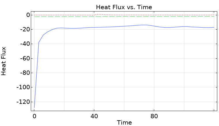
At quasi-steady state, energy in equals energy out: $Q_{in} \approx Q_{wall} + Q_{top}$
Summary: The Complete Workflow
flowchart LR
    A[Build\n Geometry] --> B[Define\n Materials]
    B --> C[Set\n Boundary Conditions]
    C --> D[Configure\n Events]
    D --> E[Generate\n Mesh]
    E --> F[Run\n Simulation]
    F --> G[Analyze\n Results]
- Build Geometry: Create 2D axisymmetric model of kettle with water domain and solid regions
- Define Materials: Assign temperature-dependent water properties and solid material properties
- Set Boundary Conditions: Configure heating plate, sidewall convection, and water surface conditions
- Configure Events: Implement thermostat hysteresis control logic
- Generate Mesh: Create structured mesh with boundary layer refinement
- Run Simulation: Execute time-dependent solver with appropriate tolerances
- Analyze Results: Examine temperature fields, flow patterns, and species distribution
Conclusions and Future Work
What We Learned
This simulation journey revealed several interesting insights:
Convection dominates: The high Rayleigh number confirms that natural convection—not conduction—is the primary heat transfer mechanism. The beautiful recirculation patterns in our streamline plots prove it.
Smart thermostat design: The hysteresis strategy works exactly as intended, keeping water within ±0.5°C of the target while avoiding the rapid on-off cycling that would plague a simple threshold controller.
Where the heat goes: Most heat escapes through the sidewalls rather than the water surface—a consequence of the larger contact area with the glass.
Mixing for free: Natural convection dramatically accelerates species transport, dispersing dissolved substances far faster than diffusion alone.
Model Limitations
No model is perfect. Ours makes several simplifying assumptions:
- 2D axisymmetric geometry (can’t capture 3D asymmetric effects)
- No evaporation at the water surface (important at higher temperatures)
- Spatially uniform heating plate temperature
- Perfect thermal contact at material interfaces
Where to Go From Here
Several exciting extensions await:
- Phase change: Add boiling and evaporation models for high-temperature operation
- Realistic heating: Model the actual Joule heating distribution in the heating element
- Full 3D: Capture asymmetric effects from handles and spouts
- Smarter control: Implement PID control for improved energy efficiency
- Surface effects: Include Marangoni convection at the water-air interface
References
- COMSOL Multiphysics Documentation - Heat Transfer Module
- COMSOL Application Gallery - Free Convection in a Water Glass
- Incropera, F.P., DeWitt, D.P., Bergman, T.L., & Lavine, A.S. Fundamentals of Heat and Mass Transfer (7th ed.). Wiley.
- COMSOL Application Gallery - Nonisothermal Flow Examples