PDE Classification: The DNA of Physics
Introduction
Before we dive into solving Partial Differential Equations (PDEs) numerically, we must first diagnose the equation. Just as a doctor treats a virus differently from a broken bone, a computational physicist uses completely different algorithms for different types of PDEs.
The classification into Elliptic, Parabolic, and Hyperbolic types isn’t arbitrary—it reflects a deep truth about the physics:
In physics, classifying PDEs is essentially distinguishing between wave propagation and particle diffusion, or equivalently, reversible and irreversible processes.
| Type | Physical Essence | The Big Question |
|---|---|---|
| Hyperbolic | Wave propagation | How fast does information travel? |
| Parabolic | Diffusion/Smoothing | How does disorder spread? |
| Elliptic | Equilibrium/Steady-state | What is the final balanced state? |
Understanding this classification is the key to choosing correct boundary conditions, initial conditions, and numerical schemes.
The Master Equation & Discriminant
Consider a general linear second-order PDE for $u(x,y)$:
$$A u_{xx} + 2B u_{xy} + C u_{yy} + \text{lower order terms} = 0$$
The discriminant determines the type:
$$\Delta = B^2 - AC$$
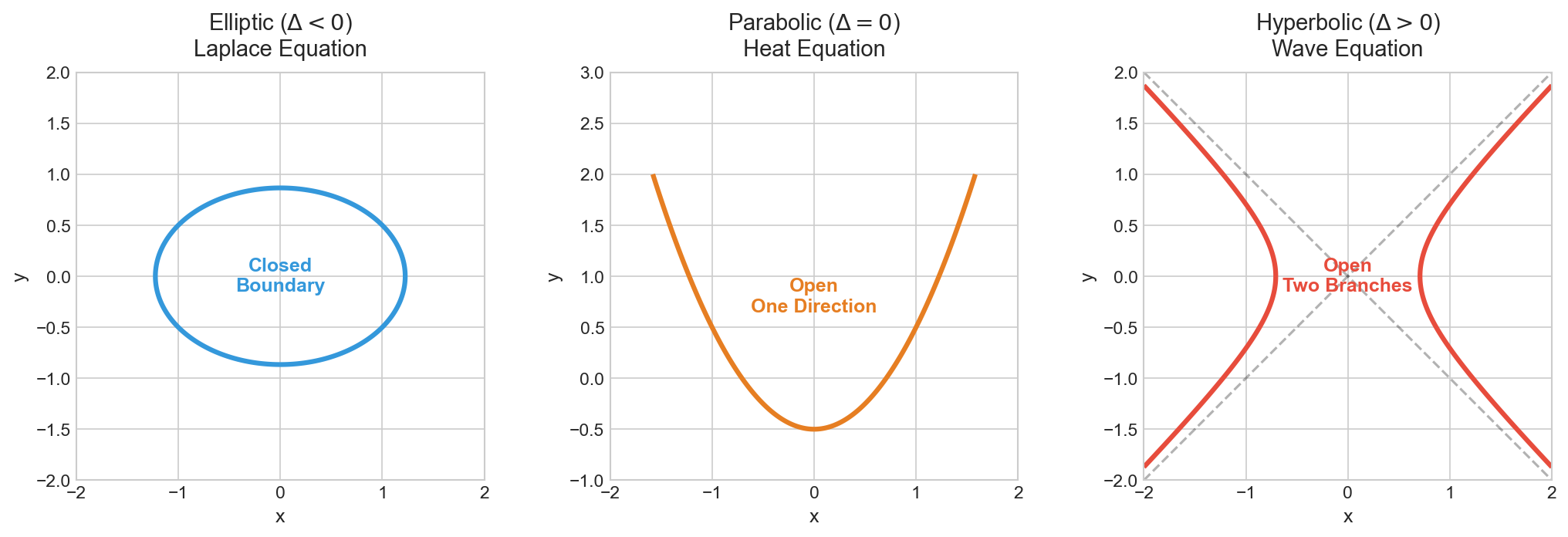
| $\Delta$ | Type | Geometry Analogy |
|---|---|---|
| $< 0$ | Elliptic | Ellipse (closed) |
| $= 0$ | Parabolic | Parabola (open, one direction) |
| $> 0$ | Hyperbolic | Hyperbola (open, two directions) |
Hyperbolic PDEs: Causality and Waves
Physical Intuition: “Information propagation takes time and has a maximum speed.”
Prototype: The Wave Equation $$\frac{\partial^2 u}{\partial t^2} = c^2 \nabla^2 u$$
Examples: Electromagnetic waves, sound waves, gravitational waves, seismic waves.
Why It Matters Physically
Finite Propagation Speed (Causality)
This is the most important physical feature. If the Sun were to suddenly vanish, Earth wouldn’t know for 8 minutes—the time it takes light to travel from the Sun to Earth. Hyperbolic equations enforce causality: information cannot spread instantaneously across space.Light Cones and Characteristics
In spacetime, hyperbolic equations divide the universe into “past,” “future,” and “elsewhere.” Disturbances can only propagate within the characteristic cone (the light cone in relativity). This is why we can’t send messages faster than light.Energy Conservation
In an ideal hyperbolic system (without damping), the wave just moves—energy is neither created nor destroyed, only transferred. This is why sound echoes and light reflects.Shock Waves and Discontinuities
Unlike parabolic equations which smooth everything out, hyperbolic equations can preserve and propagate discontinuities. Supersonic jets create sonic booms precisely because the Euler equations are hyperbolic when flow velocity exceeds the speed of sound.
Typical Physical Scenarios
- Electrodynamics: Maxwell’s equations in vacuum are hyperbolic (light waves).
- Acoustics: Sound propagation through air follows the wave equation.
- Supersonic Fluid Dynamics: When $v > c_{\text{sound}}$, the Euler equations become hyperbolic. The fluid cannot “warn” upstream obstacles, leading to shock formation.
Parabolic PDEs: Dissipation and Diffusion
Physical Intuition: “Macroscopic smoothing driven by microscopic random walks.”
Prototype: The Heat/Diffusion Equation $$\frac{\partial u}{\partial t} = D \nabla^2 u$$
Examples: Thermal conduction, Brownian motion, momentum diffusion (viscosity), chemical diffusion (Fick’s law).
Why It Matters Physically
Infinite Propagation Speed (Mathematically)
Counterintuitively, if you heat one point in a diffusion equation, the temperature at infinity becomes instantly non-zero (though exponentially small). This reflects the non-relativistic approximation inherent in the classical diffusion model. Physically, this infinite speed is not realized because molecules have finite speeds.Smoothing Effect
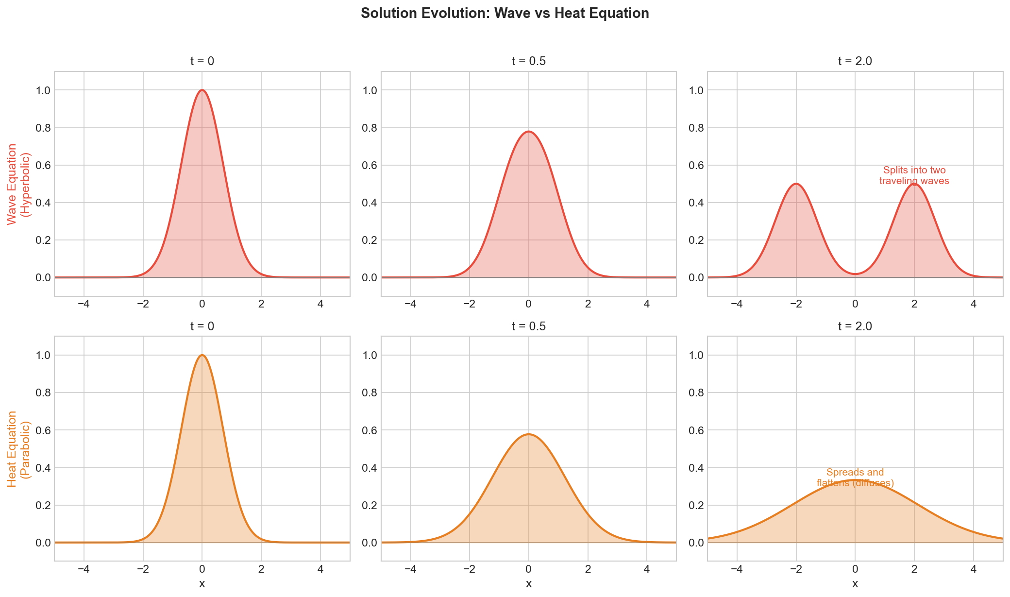
No matter how sharp the initial condition (even a Dirac delta function), the solution immediately becomes a smooth Gaussian. Physical information (fine details) gets “smeared out.” This is dissipation in action—hot coffee eventually reaches room temperature.Time Irreversibility (Entropy)
This is the Second Law of Thermodynamics in action. You can play a wave equation backwards (time-reversal symmetric), but you cannot reverse diffusion. A drop of ink in water will never spontaneously reassemble—“entropy always increases.”
Typical Physical Scenarios
- Transport Phenomena: Fick’s law for mass diffusion, Fourier’s law for heat conduction.
- Fluid Mechanics (Boundary Layers): The viscous term $\nu \nabla^2 \mathbf{v}$ in Navier-Stokes is parabolic. It causes energy dissipation and creates boundary layers.
The Schrödinger equation $i\hbar \frac{\partial \psi}{\partial t} = \hat{H}\psi$ looks parabolic (first-order in time), but the imaginary $i$ changes everything—wavefunctions oscillate, probability is conserved, and the process is reversible. Mathematically, it behaves more like a hyperbolic equation!
Elliptic PDEs: Equilibrium and Global Balance
Physical Intuition: “Everything is connected; disturbances are felt everywhere instantly.”
Prototype: The Laplace/Poisson Equation $$\nabla^2 u = 0 \quad \text{(Laplace)} \\ \nabla^2 u = f \quad \text{(Poisson)}$$
Examples: Steady-state temperature distribution, electrostatic potential, incompressible fluid flow, gravitational potential.
Why It Matters Physically
Global Dependence
Every point influences every other point. If you change the voltage on one boundary of a conductive plate, the electric potential changes everywhere inside simultaneously to reach a new equilibrium. There is no “propagation”—it’s an instantaneous global adjustment.Maximum Principle
Solutions cannot have local maxima or minima inside the domain; extrema must occur on the boundaries. This is like a stretched rubber membrane—push anywhere, and the entire surface adjusts smoothly.Infinite Smoothness
Elliptic solutions are analytic (infinitely differentiable) in the interior, even if boundary conditions are rough. Nature “smooths out” any irregularities.Mean Value Property
For harmonic functions (solutions to Laplace’s equation), the value at any point equals the average of values on any surrounding sphere. This is why elliptic solutions have no interior extrema.
Typical Physical Scenarios
- Electrostatics: The electric potential in a charge-free region satisfies Laplace’s equation.
- Steady-State Heat: When $\partial T / \partial t = 0$, the heat equation reduces to the Laplace equation.
- Incompressible Flow: The velocity potential of irrotational flow satisfies Laplace’s equation.
Summary: The Physics Table
| Feature | Hyperbolic | Parabolic | Elliptic |
|---|---|---|---|
| Represents | Waves (Light, Sound) | Diffusion (Heat, Ink) | Equilibrium (Potential) |
| Mechanism | Inertia + Restoring force | Random collisions, statistics | Global balance |
| Information Speed | Finite ($c$, light cone) | Infinite (mathematically) | Instantaneous (steady-state) |
| Smoothness | Preserves shocks | Smooths everything | Already smooth |
| Time Reversibility | Reversible (energy conserved) | Irreversible (entropy ↑) | N/A (no time) |
| Initial Conditions | $u$ and $\frac{\partial u}{\partial t}$ required | Only $u$ required | N/A (boundary-value problem) |
| Fluid Mechanics | Supersonic flow | Viscous diffusion/BL | Incompressible |

When coefficients $A, B, C$ depend on position or the solution itself, the PDE type can change across the domain. A classic example is transonic flow: subsonic regions are elliptic, supersonic regions are hyperbolic, and the sonic line ($M=1$) is where the transition occurs. This is why transonic aerodynamics is notoriously difficult!
Why Does This Classification Matter?
Choosing Initial/Boundary Conditions
- Hyperbolic: You need both the initial position $u(x, 0)$ and initial velocity $\frac{\partial u}{\partial t}(x, 0)$. Think of a guitar string: you need to know its shape and how it’s moving.
- Parabolic: You only need the initial distribution $u(x, 0)$. The rate of change is determined by the physics.
- Elliptic: No initial conditions! Only boundary conditions matter. This is a steady-state problem.
Numerical Stability
If you use a heat equation algorithm to solve the wave equation, your simulation will explode (numerical instability). The CFL condition, implicit vs. explicit schemes, and choice of solver all depend fundamentally on understanding what type of equation you’re dealing with.
References
- Evans, L. C. (2010). Partial Differential Equations (2nd ed.). American Mathematical Society.
- Strikwerda, J. C. (2004). Finite Difference Schemes and Partial Differential Equations (2nd ed.). SIAM.
- Courant, R., & Hilbert, D. (1962). Methods of Mathematical Physics, Vol. II: Partial Differential Equations. Wiley-Interscience.