ML-12: SVM: Kernel Methods and Soft Margin

Publish on: 2022/04/17 Classify at: CODE/Supervised Machine Learning

Words: 2454 Read:≈ 12min

Summary

Go beyond linear SVM: master the kernel trick for nonlinear boundaries, understand RBF and polynomial kernels, and learn soft-margin SVM with the C parameter for handling real-world noisy data.

Learning Objectives

Understand the kernel trick
Use polynomial and RBF kernels
Implement soft-margin SVM
Tune hyperparameter C

Theory

The Problem: When Linear Isn’t Enough

In last blog, hard-margin SVM was introduced to find linear decision boundaries. But what if data looks like this?

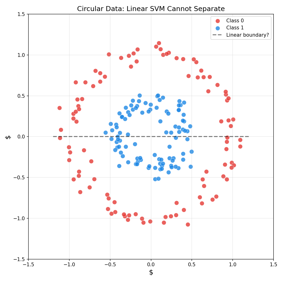
Circular data example — Circular data: no linear boundary can separate the inner ring (red) from the outer ring (blue).

For data with circular, spiral, or other complex patterns, no linear hyperplane can separate the classes. Nonlinear decision boundaries are required.

The Kernel Trick: The Big Idea

Feature Mapping φ(x)

One solution: transform the data to a higher-dimensional space where it becomes linearly separable.

Example: For circular data in 2D, map $(x_1, x_2)$ to 3D:

$$\phi(x) = (x_1^2, \sqrt{2}x_1 x_2, x_2^2)$$

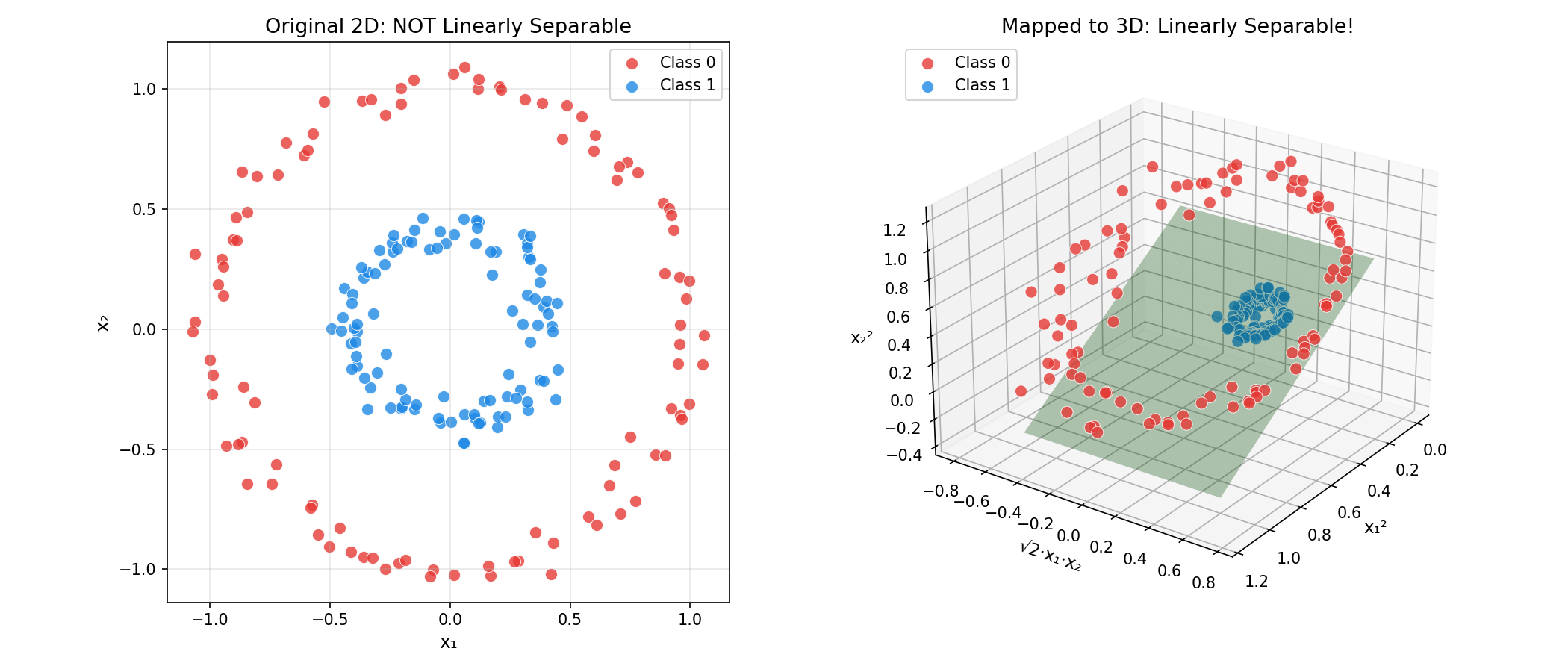
Feature mapping visualization — Left: 2D circular data cannot be linearly separated. Right: After mapping to 3D with φ(x), a flat plane (green) separates the classes!

In this new space, the circular boundary becomes a flat plane!

The Computational Problem

But there’s a catch: if we map to a very high-dimensional space (or even infinite dimensions), computing $\phi(x)$ explicitly is expensive or impossible.

The Kernel Trick Solution

Recall from the dual formulation, the optimization only involves dot products $x_i^T x_j$.

Key insight: We can compute the dot product in the transformed space without explicitly computing $\phi(x)$:

$$K(x_i, x_j) = \phi(x_i)^T \phi(x_j)$$

This is the kernel function — it computes the inner product in high-dimensional space using only the original features!

Why this works: The kernel function is a “shortcut” that gives the same result as:

Transform $x_i$ and $x_j$ to high dimensions
Compute their dot product

But step 1 is skipped entirely!

Common Kernels

Linear Kernel

$$K(x_i, x_j) = x_i^T x_j$$

What it does: No transformation, equivalent to standard SVM
When to use: Data is already linearly separable
Advantage: Fastest, least prone to overfitting

Polynomial Kernel

$$K(x_i, x_j) = (\gamma \cdot x_i^T x_j + r)^d$$

where $d$ is the degree, $r$ is the coefficient (coef0), and $\gamma$ scales the dot product.

Geometric intuition:

$d = 2$: Can learn elliptical and parabolic boundaries
$d = 3$: Can learn cubic curves
Higher $d$: More complex shapes (but risk overfitting)

Parameter	Effect
`degree`	Polynomial degree — higher = more flexible
`coef0`	Shifts the polynomial (affects shape)
`gamma`	Scales input features

In practice: Degree 2-3 is usually sufficient. Higher degrees often overfit.

RBF (Radial Basis Function) Kernel

$$K(x_i, x_j) = \exp\left(-\gamma |x_i - x_j|^2\right)$$

Also called the Gaussian kernel. This is the most popular kernel!

Geometric intuition:

Measures similarity between points
Points close together → $K \approx 1$
Points far apart → $K \approx 0$

The magic: RBF implicitly maps to an infinite-dimensional space! Yet we compute it with a simple formula.

The γ (Gamma) Parameter

γ Value	Effect	Risk
High γ	Each point has very local influence	Overfitting (complex, wiggly boundary)
Low γ	Points influence far away	Underfitting (too smooth boundary)

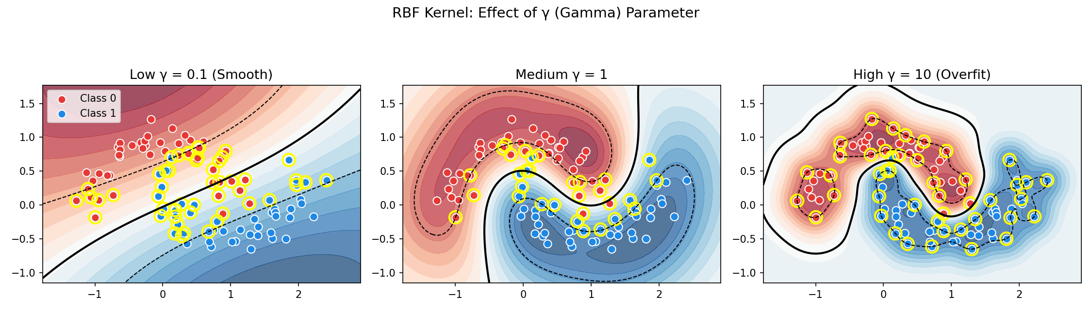
RBF gamma parameter comparison — Effect of γ: Low γ produces smooth boundaries, high γ creates tight, complex boundaries that overfit.

Common mistake: Using default gamma='scale' without checking. Always visualize or cross-validate!

Soft Margin SVM: Handling Noise

Why Hard Margin Fails

Real-world data is messy:

Outliers that cross the margin
Overlapping classes with no clean separation
Noise that makes perfect separation impossible

Hard-margin SVM will either:

Fail completely (no solution)
Find a terrible boundary trying to fit outliers

The Solution: Allow Some Mistakes

Introduce slack variables $\xi_i \geq 0$ that measure how much each point violates the margin:

$$y_i(w^T x_i + b) \geq 1 - \xi_i$$

$\xi_i$ Value	Meaning
$\xi_i = 0$	Point is on or outside the margin (correct)
$0 < \xi_i < 1$	Point is inside the margin but correct side
$\xi_i \geq 1$	Point is misclassified

The Soft-Margin Optimization Problem

Minimize:

$$\boxed{\frac{1}{2}|w|^2 + C \sum_{i=1}^{N} \xi_i}$$

Subject to:

$y_i(w^T x_i + b) \geq 1 - \xi_i, \quad \forall i$
$\xi_i \geq 0, \quad \forall i$

The objective balances:

$\dfrac{1}{2}|w|^2$ — maximize margin (as before)
$C \sum \xi_i$ — penalize violations

The C Parameter: Bias-Variance Tradeoff

$C$ controls how much we penalize margin violations:

C Value	Margin	Errors	Behavior
Large C	Narrow	Few allowed	Low bias, high variance — fits training data tightly
Small C	Wide	More allowed	High bias, low variance — smoother, more generalizable

Rule of thumb:

Start with C=1 and adjust based on cross-validation
If overfitting → decrease C
If underfitting → increase C

Soft-Margin Dual Problem

The dual becomes:

$$\max_\alpha \sum_{i=1}^{N} \alpha_i - \frac{1}{2} \sum_{i,j} \alpha_i \alpha_j y_i y_j K(x_i, x_j)$$

Subject to:

$0 \leq \alpha_i \leq C, \quad \forall i$ (the box constraint!)
$\sum_{i=1}^{N} \alpha_i y_i = 0$

The only difference from hard-margin: $\alpha_i$ is now bounded by C instead of just $\alpha_i \geq 0$.

Three Types of Points

After training, each point falls into one category:

Condition	Type	Role
$\alpha_i = 0$	Non-support vector	Far from boundary, doesn’t affect model
$0 < \alpha_i < C$	Free support vector	Exactly on the margin
$\alpha_i = C$	Bounded support vector	Inside margin or misclassified

Code Practice

The following examples demonstrate kernels and soft margins in action.

Comparing Kernels on Circular Data

This example shows why kernel choice matters. The make_circles data creates concentric rings — impossible to separate linearly.

🐍 Python

 1
 2
 3
 4
 5
 6
 7
 8
 9
10
11
12
13
14
15
16
17
18
19
20
21
22
23
24
25
26
27
28
29
30
31
32
33
34
35
36
37
38
39
40
41
42
43
44
45
46
47
48
49
50
51
52
53
54
55
56
57
58
59
60
import numpy as np
import matplotlib.pyplot as plt
from sklearn.svm import SVC
from sklearn.datasets import make_circles

# Generate non-linearly separable data (concentric circles)
X, y = make_circles(n_samples=200, noise=0.1, factor=0.3, random_state=42)
y = np.where(y == 0, -1, 1)  # Convert to {-1, +1}

fig, axes = plt.subplots(1, 3, figsize=(15, 4.5))
kernels = ['linear', 'poly', 'rbf']
results = []

for ax, kernel in zip(axes, kernels):
    # Train SVM with specified kernel
    svm = SVC(kernel=kernel, C=1, degree=3, gamma='auto')
    svm.fit(X, y)
    
    # Create decision boundary visualization
    xx, yy = np.meshgrid(np.linspace(-1.5, 1.5, 200),
                         np.linspace(-1.5, 1.5, 200))
    Z = svm.decision_function(np.c_[xx.ravel(), yy.ravel()])
    Z = Z.reshape(xx.shape)
    
    # Plot with gradient effect
    ax.contourf(xx, yy, Z, levels=np.linspace(Z.min(), Z.max(), 20), 
                cmap='RdBu', alpha=0.7)
    ax.contour(xx, yy, Z, levels=[0], colors='black', linewidths=2)
    ax.contour(xx, yy, Z, levels=[-1, 1], colors='black', 
               linewidths=1, linestyles='dashed')
    
    # Plot data points
    ax.scatter(X[y==1, 0], X[y==1, 1], c='#1E88E5', s=60, 
               edgecolors='white', label='Class +1')
    ax.scatter(X[y==-1, 0], X[y==-1, 1], c='#E53935', s=60, 
               edgecolors='white', label='Class -1')
    
    # Highlight support vectors
    ax.scatter(svm.support_vectors_[:, 0], svm.support_vectors_[:, 1],
               s=150, facecolors='none', edgecolors='yellow', linewidths=2)
    
    acc = svm.score(X, y)
    n_sv = len(svm.support_vectors_)
    ax.set_title(f'{kernel.upper()}\nAccuracy: {acc:.0%} | SVs: {n_sv}')
    ax.set_xlim(-1.5, 1.5)
    ax.set_ylim(-1.5, 1.5)
    ax.grid(True, alpha=0.3)
    results.append((kernel, acc, n_sv))

axes[0].legend(loc='upper right')
fig.suptitle('Kernel Comparison on Circular Data', fontsize=14)
plt.tight_layout(rect=[0, 0, 1, 0.95])
plt.savefig('assets/kernels.png', dpi=150, facecolor='white')
plt.show()

# Print comparison
print("\n📊 Kernel Comparison Results:")
print("-" * 40)
for kernel, acc, n_sv in results:
    print(f"  {kernel.upper():10s} | Accuracy: {acc:5.1%} | SVs: {n_sv}")

Output:

Kernel comparison on circular data — Kernel comparison: only RBF achieves perfect separation on concentric circle data.

1
2
3
4
5
📊 Kernel Comparison Results:
----------------------------------------
  LINEAR     | Accuracy: 66.0% | SVs: 200
  POLY       | Accuracy: 64.5% | SVs: 200
  RBF        | Accuracy: 100.0% | SVs: 45

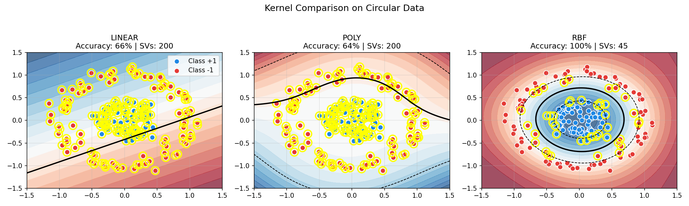
Key observations:

Linear and Polynomial kernels fail on circular data (~65%)
RBF achieves perfect separation (100%) by mapping to infinite dimensions
More support vectors indicate a more complex decision boundary

Effect of C Parameter (Soft Margin)

The following visualization shows how C affects the decision boundary on noisy data:

🐍 Python

 1
 2
 3
 4
 5
 6
 7
 8
 9
10
11
12
13
14
15
16
17
18
19
20
21
22
23
24
25
26
27
28
29
30
31
32
33
34
35
36
37
38
39
40
41
42
43
44
45
46
47
48
49
50
51
52
53
54
from sklearn.datasets import make_moons

fig, axes = plt.subplots(1, 3, figsize=(15, 4.5))
C_values = [0.01, 1, 100]

# Generate moon-shaped data with noise (better shows C effect)
X, y = make_moons(n_samples=150, noise=0.2, random_state=42)
y = np.where(y == 0, -1, 1)  # Convert to {-1, +1}

results_c = []
for ax, C in zip(axes, C_values):
    svm = SVC(kernel='rbf', C=C, gamma=2)  # Fixed gamma to isolate C effect
    svm.fit(X, y)
    
    xx, yy = np.meshgrid(np.linspace(X[:, 0].min()-0.5, X[:, 0].max()+0.5, 200),
                         np.linspace(X[:, 1].min()-0.5, X[:, 1].max()+0.5, 200))
    Z = svm.decision_function(np.c_[xx.ravel(), yy.ravel()])
    Z = Z.reshape(xx.shape)
    
    # Plot with gradient effect
    ax.contourf(xx, yy, Z, levels=np.linspace(Z.min(), Z.max(), 20), 
                cmap='RdBu', alpha=0.7)
    ax.contour(xx, yy, Z, levels=[0], colors='black', linewidths=2)
    ax.contour(xx, yy, Z, levels=[-1, 1], colors='black', 
               linewidths=1, linestyles='dashed')
    
    # Plot data points
    ax.scatter(X[y==1, 0], X[y==1, 1], c='#1E88E5', s=60, 
               edgecolors='white', label='Class +1')
    ax.scatter(X[y==-1, 0], X[y==-1, 1], c='#E53935', s=60, 
               edgecolors='white', label='Class -1')
    
    # Highlight support vectors
    ax.scatter(svm.support_vectors_[:, 0], svm.support_vectors_[:, 1],
               s=150, facecolors='none', edgecolors='yellow', linewidths=2)
    
    acc = svm.score(X, y)
    n_sv = len(svm.support_vectors_)
    ax.set_title(f'C={C}\nAccuracy: {acc:.0%} | SVs: {n_sv}')
    ax.grid(True, alpha=0.3)
    results_c.append((C, acc, n_sv))

axes[0].legend(loc='upper right')
fig.suptitle('Effect of C Parameter (Regularization)', fontsize=14)
plt.tight_layout(rect=[0, 0, 1, 0.95])
plt.savefig('assets/soft_margin.png', dpi=150, facecolor='white')
plt.show()

print("\n📊 C Parameter Effect:")
print("-" * 50)
print(f"{'C':>8} | {'Accuracy':>10} | {'Support Vectors':>16}")
print("-" * 50)
for C, acc, n_sv in results_c:
    print(f"{C:>8} | {acc:>10.1%} | {n_sv:>16}")

Output:

C parameter effect on decision boundary — Effect of C: Low C allows more margin violations (smooth), high C enforces stricter classification (complex boundary).

1
2
3
4
5
6
7
📊 C Parameter Effect:
--------------------------------------------------
       C |   Accuracy |  Support Vectors
--------------------------------------------------
    0.01 |      89.3% |              150
       1 |      96.0% |               43
     100 |      97.3% |               21

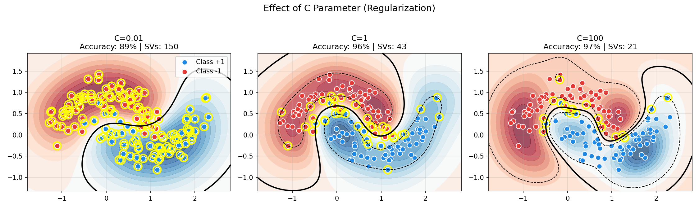
Observe the tradeoff:

Low C (soft margin): Smooth boundary, many support vectors, tolerates misclassification
High C (hard margin): Complex boundary, fewer support vectors, fits noise
Balanced C: Best generalization on noisy data

Grid Search for Hyperparameters

Always use cross-validation to find optimal C and γ:

🐍 Python

 1
 2
 3
 4
 5
 6
 7
 8
 9
10
11
12
13
14
15
16
17
18
19
20
21
22
23
24
25
26
27
28
29
30
from sklearn.model_selection import GridSearchCV, cross_val_score
import pandas as pd

# Define parameter grid
param_grid = {
    'C': [0.1, 1, 10, 100],
    'gamma': ['scale', 'auto', 0.1, 1],
    'kernel': ['rbf', 'poly']
}

# Grid search with 5-fold cross-validation
svm = SVC()
grid = GridSearchCV(svm, param_grid, cv=5, scoring='accuracy', 
                    return_train_score=True)
grid.fit(X, y)

print("🔍 Grid Search Results")
print("=" * 50)
print(f"\n✅ Best Parameters: {grid.best_params_}")
print(f"📈 Best CV Score:   {grid.best_score_:.2%}")

# Show top 5 configurations
print("\n📊 Top 5 Configurations:")
results_df = pd.DataFrame(grid.cv_results_)
top5 = results_df.nsmallest(5, 'rank_test_score')[
    ['param_kernel', 'param_C', 'param_gamma', 'mean_test_score']
]
for _, row in top5.iterrows():
    print(f"   {row['param_kernel']:5s} | C={row['param_C']:>4} | "
          f"γ={str(row['param_gamma']):>6s} | Score: {row['mean_test_score']:.2%}")

Output:

 1
 2
 3
 4
 5
 6
 7
 8
 9
10
11
12
🔍 Grid Search Results
==================================================

✅ Best Parameters: {'C': 10, 'gamma': 'scale', 'kernel': 'rbf'}
📈 Best CV Score:   96.00%

📊 Top 5 Configurations:
   rbf   | C=10.0 | γ= scale | Score: 96.00%
   rbf   | C=10.0 | γ=     1 | Score: 96.00%
   rbf   | C=100.0 | γ=  auto | Score: 95.33%
   rbf   | C=100.0 | γ= scale | Score: 94.00%
   rbf   | C=100.0 | γ=     1 | Score: 94.00%

Grid search tips: Start with coarse values (C: 0.1–100, γ: scale/auto), then refine. For large spaces, use RandomizedSearchCV.

Deep Dive

Frequently Asked Questions

Q1: How do I choose between kernels?

Start with this decision flowchart:

graph TD A["🎯 Start"] --> B{"Linearly<br/>separable?"} B -->|Yes| C["✅ Linear Kernel"] B -->|No| D{"Know pattern?"} D -->|"Polynomial"| E["📐 Polynomial"] D -->|"Unknown"| F["🔮 RBF Kernel"] E -->|"Underfit"| F F --> G["⚙️ Tune C & γ"] style C fill:#c8e6c9 style E fill:#fff9c4 style F fill:#bbdefb style G fill:#e1bee7

Data Characteristics	Recommended Kernel	Why
High-dim text/documents	Linear	Features are already expressive; linear is fast
Low-dim with clear curves	Polynomial (d=2-3)	Can fit ellipses, parabolas
Complex, unknown structure	RBF	Universal approximator
Very large dataset	Linear or Approx. RBF	RBF is $O(n^2)$

Q2: What does γ (gamma) really do?

γ controls the “reach” of each training point’s influence:

$$K(x_i, x_j) = \exp(-\gamma |x_i - x_j|^2)$$

γ Value	Influence Radius	Decision Boundary	Risk
Very high (e.g., 100)	Tiny	Wiggly, fits every point	Severe overfitting
High (e.g., 10)	Small	Complex, detailed	Overfitting
Medium (e.g., 1)	Moderate	Balanced	-
Low (e.g., 0.1)	Large	Smooth	Underfitting
Very low (e.g., 0.01)	Huge	Nearly linear	Severe underfitting

Quick intuition: γ = 1/(2σ²) where σ is the “width” of the Gaussian. Higher γ = narrower Gaussian = more local influence.

Q3: How do C and γ interact?

Both affect model complexity, but in different ways:

Parameter	Controls	Too Low	Too High
C	Penalty for misclassification	Underfitting (too smooth)	Overfitting (fits outliers)
γ	Locality of influence	Underfitting (too smooth)	Overfitting (too complex)

Practical tuning strategy:

Fix γ='scale' (sklearn default), tune C first
Then tune γ with best C
Or use 2D grid search from the start:
- C: [0.1, 1, 10, 100, 1000]
- γ: [0.001, 0.01, 0.1, 1, 10]

Q4: Why is my SVM slow?

Symptom	Cause	Solution
Training takes forever	Large N with RBF kernel	Use `LinearSVC` or reduce data
Many support vectors	C too small or data overlaps	Increase C or use linear kernel
Prediction is slow	Too many SVs	Reduce SVs via regularization

RBF scaling: Training time is approximately $O(n^2)$ to $O(n^3)$. For >10,000 samples, consider:

LinearSVC (much faster)
SGDClassifier with kernel approximation
Subsampling the training data

Kernel Selection Guide

Domain	Typical Kernel	Reason
Text Classification	Linear	TF-IDF features are high-dimensional and often linearly separable
Image Classification	RBF or CNN	Pixel relationships are complex
Genomics	Linear or String kernels	High-dimensional sparse features
Time Series	RBF or custom	Depends on the distance metric
Financial Data	RBF	Often has complex nonlinear patterns

Hyperparameter Tuning Strategies

Coarse-to-Fine Search

1
2
3
4
5
6
7
8
# Step 1: Coarse search (logarithmic scale)
C_range = [0.01, 0.1, 1, 10, 100, 1000]
gamma_range = [0.0001, 0.001, 0.01, 0.1, 1, 10]

# Step 2: Fine search around best values
# If best was C=10, gamma=0.1:
C_fine = [5, 7, 10, 15, 20]
gamma_fine = [0.05, 0.08, 0.1, 0.12, 0.15]

Common Pitfalls

Pitfall	Symptom	Solution
Not scaling features	Poor performance, sensitive to feature magnitude	Always use `StandardScaler`
Using RBF on linearly separable data	Slow training, similar accuracy to linear	Try linear kernel first
Overfitting with high C and γ	Great train accuracy, poor test accuracy	Use cross-validation, reduce C/γ
Default γ=‘scale’ on unnormalized data	Unpredictable results	Scale data first, then use defaults
Grid search on entire dataset	Optimistic bias	Use nested cross-validation

When NOT to Use SVM

Scenario	Better Alternative
Very large datasets (N > 100k)	Gradient boosting, neural networks
Need probability outputs	Logistic regression, calibrated SVM
Many noisy features	Random forest (automatic feature selection)
Online learning required	SGDClassifier
Interpretability critical	Decision trees, logistic regression

Summary

Concept	Key Points
Kernel Trick	Implicit high-dim mapping via $K(x_i, x_j)$
RBF Kernel	$\exp(-\gamma\|x_i - x_j\|^2)$ — most flexible
Soft Margin	Allows $\xi_i$ slack for misclassifications
C Parameter	Tradeoff margin width vs errors

References

Boser, B. et al. (1992). “A Training Algorithm for Optimal Margin Classifiers”
sklearn Kernel SVM Tutorial
Schölkopf, B. & Smola, A. “Learning with Kernels”