Learning Objectives

• Understand why logistic regression is needed for classification
• Master the sigmoid function
• Derive cross-entropy loss
• Handle multi-class problems

Theory

From Linear to Logistic

Classification tasks differ fundamentally from regression. Consider spam detection: given email features, the goal is to predict whether an email is spam (1) or not spam (0).

The Problem with Linear Regression:

If linear regression is applied directly: $$\hat{y} = \boldsymbol{w}^T \boldsymbol{x}$$

The output can be any real number: $-\infty$ to $+\infty$. But for classification:

• A probability between 0 and 1 is needed
• A clear decision rule is required (e.g., if probability > 0.5, predict class 1)

The Solution: A function that “squashes” any real number into the (0, 1) range solves this problem — enter the sigmoid function.

Sigmoid Function

$$\sigma(z) = \frac{1}{1 + e^{-z}}$$

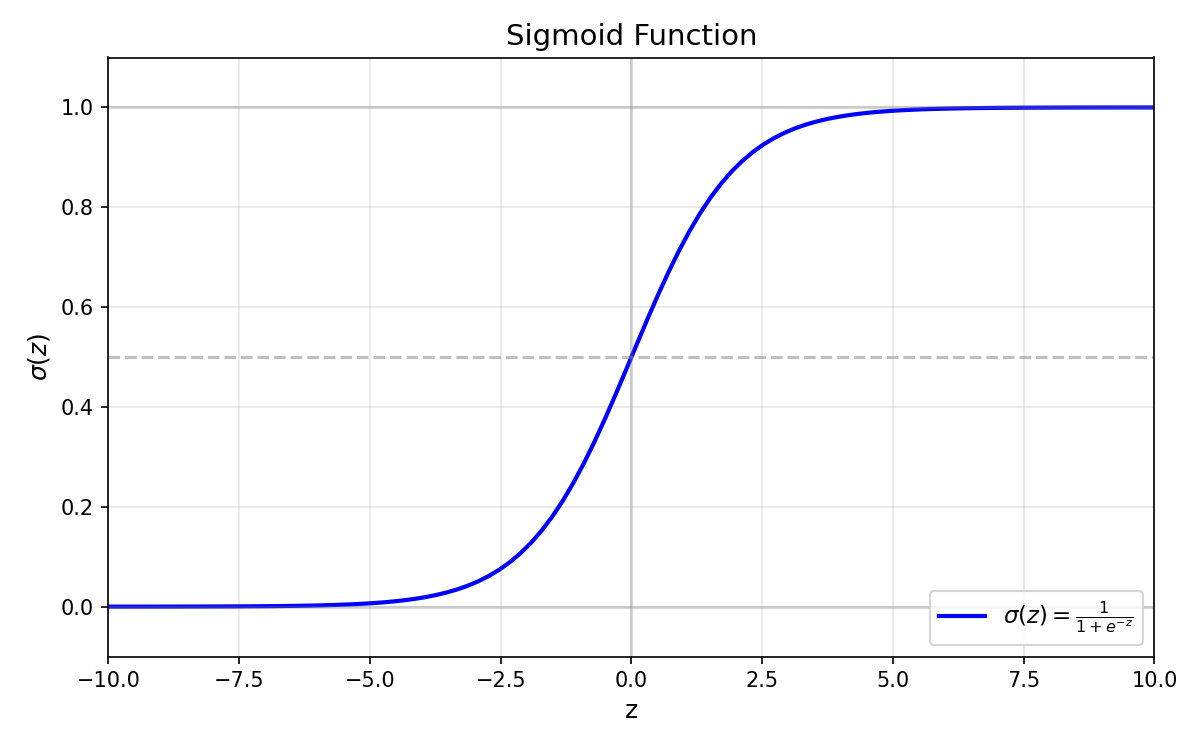
Key Properties:

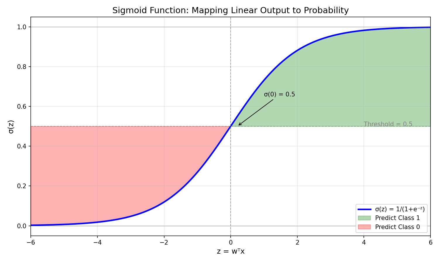
Why Sigmoid?

1. Probabilistic interpretation: Output can be interpreted as $P(y=1|x)$
2. Smooth gradients: Unlike step functions, sigmoid is differentiable everywhere — essential for gradient-based optimization
3. Natural decision boundary: The 0.5 threshold corresponds to $\boldsymbol{w}^T \boldsymbol{x} = 0$

Logistic Regression Model

With the sigmoid function in hand, the logistic regression model combines linear combination with probability transformation:

$$P(y=1|\boldsymbol{x}) = \sigma(\boldsymbol{w}^T \boldsymbol{x}) = \frac{1}{1 + e^{-\boldsymbol{w}^T \boldsymbol{x}}}$$

Decision Rule:

• If $P(y=1|\boldsymbol{x}) \geq 0.5$ → predict class 1
• If $P(y=1|\boldsymbol{x}) < 0.5$ → predict class 0

This is equivalent to:

• If $\boldsymbol{w}^T \boldsymbol{x} \geq 0$ → predict class 1
• If $\boldsymbol{w}^T \boldsymbol{x} < 0$ → predict class 0

The equation $\boldsymbol{w}^T \boldsymbol{x} = 0$ defines the decision boundary — a hyperplane that separates the two classes.

Cross-Entropy Loss

To train the model, a loss function that measures prediction quality is needed.

Why not Mean Squared Error (MSE)? For probability outputs, MSE produces flat gradients near 0 and 1, making learning slow. Cross-entropy provides stronger gradients for wrong predictions, enabling faster and more effective learning.

Derivation from Maximum Likelihood:

For a single sample with true label $y$ and predicted probability $\hat{y}$:

$$P(y|\boldsymbol{x}) = \hat{y}^y \cdot (1-\hat{y})^{(1-y)}$$

Taking the negative log (to convert maximization to minimization):

$$-\log P(y|\boldsymbol{x}) = -[y \log(\hat{y}) + (1-y)\log(1-\hat{y})]$$

For $N$ samples, the binary cross-entropy loss is:

$$L = -\frac{1}{N}\sum_{i=1}^{N}[y_i \log(\hat{y}_i) + (1-y_i)\log(1-\hat{y}_i)]$$

Intuition:

• When $y=1$: Loss = $-\log(\hat{y})$ → penalizes low predicted probability
• When $y=0$: Loss = $-\log(1-\hat{y})$ → penalizes high predicted probability

Gradient Derivation

To update the weights during training, the gradient of the loss with respect to weights must be computed. Remarkably, the math simplifies to:

$$\frac{\partial L}{\partial \boldsymbol{w}} = \frac{1}{N} \sum_{i=1}^{N} (\hat{y}_i - y_i) \boldsymbol{x}_i$$

This elegant result — simply the prediction error multiplied by the input — makes implementation straightforward and computationally efficient.

Multi-Class: One-vs-Rest (OvR)

Logistic regression naturally handles binary classification. For problems with $K > 2$ classes, the One-vs-Rest (OvR) strategy trains $K$ separate binary classifiers:

Prediction: For a new sample, run all $K$ classifiers and choose the class with highest probability.

Alternative: Softmax (Multinomial)

Rather than training $K$ separate classifiers, a more unified approach uses a single model with softmax activation:

$$P(y=k \vert \mathbf{x}) = \frac{e^{\mathbf{w}_k^T \mathbf{x}}}{\sum_{j=1}^{K} e^{\mathbf{w}_j^T \mathbf{x}}}$$

This ensures all class probabilities sum to 1.

Code Practice

This section applies the theoretical concepts to real data, starting with the classic Iris dataset and progressing through sigmoid visualization, custom implementation, and sklearn usage.

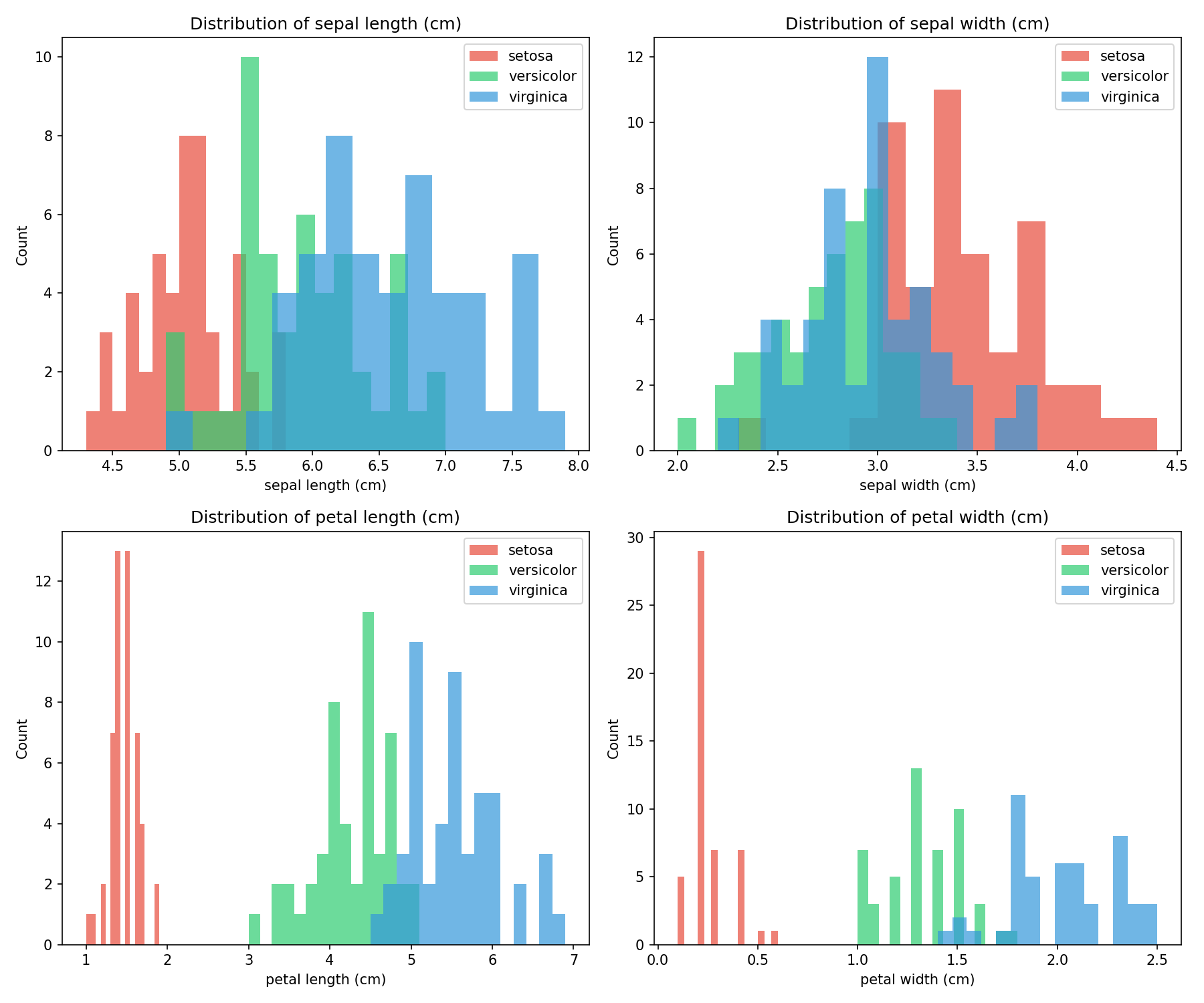
The Iris Dataset

The Iris dataset serves as a classic machine learning benchmark, containing measurements from 150 iris flowers across 3 species:

• Setosa (class 0)
• Versicolor (class 1)
• Virginica (class 2)

Each flower has 4 features: sepal length, sepal width, petal length, and petal width (all in cm).

 1
 2
 3
 4
 5
 6
 7
 8
 9
10
11
12
13
14
15

import numpy as np
import matplotlib.pyplot as plt
from sklearn.datasets import load_iris
import pandas as pd

# Load dataset
iris = load_iris()
df = pd.DataFrame(iris.data, columns=iris.feature_names)
df['species'] = [iris.target_names[i] for i in iris.target]

# Display sample
print("Iris Dataset Sample:")
print(df.head(10))
print(f"\nTotal samples: {len(df)}")
print(f"Classes: {list(iris.target_names)}")

Output:

 1
 2
 3
 4
 5
 6
 7
 8
 9
10
11
12
13
14
15
16
17

Iris Dataset Sample:
   sepal length (cm)  sepal width (cm)  ...  petal width (cm)  species
0                5.1               3.5  ...               0.2   setosa
1                4.9               3.0  ...               0.2   setosa
2                4.7               3.2  ...               0.2   setosa
3                4.6               3.1  ...               0.2   setosa
4                5.0               3.6  ...               0.2   setosa
5                5.4               3.9  ...               0.4   setosa
6                4.6               3.4  ...               0.3   setosa
7                5.0               3.4  ...               0.2   setosa
8                4.4               2.9  ...               0.2   setosa
9                4.9               3.1  ...               0.1   setosa

[10 rows x 5 columns]

Total samples: 150
Classes: [np.str_('setosa'), np.str_('versicolor'), np.str_('virginica')]

 1
 2
 3
 4
 5
 6
 7
 8
 9
10
11
12
13
14
15
16

fig, axes = plt.subplots(2, 2, figsize=(12, 10))
colors = ['#e74c3c', '#2ecc71', '#3498db']

for idx, (ax, feature) in enumerate(zip(axes.flat, iris.feature_names)):
    for i, species in enumerate(iris.target_names):
        mask = iris.target == i
        ax.hist(iris.data[mask, idx], bins=15, alpha=0.7, 
                label=species, color=colors[i])
    ax.set_xlabel(feature)
    ax.set_ylabel('Count')
    ax.legend()
    ax.set_title(f'Distribution of {feature}')

plt.tight_layout()
plt.savefig('assets/iris_distribution.png', dpi=150)
plt.show()

Sigmoid Visualization

 1
 2
 3
 4
 5
 6
 7
 8
 9
10
11
12
13
14
15
16
17
18
19
20
21
22
23
24
25
26
27
28
29
30
31
32
33
34
35
36
37
38

import numpy as np
import matplotlib.pyplot as plt

z = np.linspace(-6, 6, 200)
sigmoid = 1 / (1 + np.exp(-z))

fig, ax = plt.subplots(figsize=(10, 6))

# Main sigmoid curve
ax.plot(z, sigmoid, 'b-', linewidth=2.5, label='σ(z) = 1/(1+e⁻ᶻ)')

# Fill regions for classification
ax.fill_between(z, sigmoid, 0.5, where=(sigmoid >= 0.5), 
                alpha=0.3, color='green', label='Predict Class 1')
ax.fill_between(z, sigmoid, 0.5, where=(sigmoid < 0.5), 
                alpha=0.3, color='red', label='Predict Class 0')

# Reference lines
ax.axhline(0.5, color='gray', linestyle='--', linewidth=1, alpha=0.7)
ax.axhline(0, color='gray', linewidth=0.5)
ax.axhline(1, color='gray', linewidth=0.5)
ax.axvline(0, color='gray', linestyle='--', linewidth=1, alpha=0.7)

# Annotations
ax.annotate('Threshold = 0.5', xy=(4, 0.5), fontsize=10, color='gray')
ax.annotate('σ(0) = 0.5', xy=(0.2, 0.5), xytext=(1, 0.65),
            arrowprops=dict(arrowstyle='->', color='black'), fontsize=10)

ax.set_xlabel('z = wᵀx', fontsize=12)
ax.set_ylabel('σ(z)', fontsize=12)
ax.set_title('Sigmoid Function: Mapping Linear Output to Probability', fontsize=14)
ax.legend(loc='lower right')
ax.set_xlim(-6, 6)
ax.set_ylim(-0.05, 1.05)
ax.grid(alpha=0.3)
plt.tight_layout()
plt.savefig('assets/sigmoid.png', dpi=150)
plt.show()

Logistic Regression from Scratch

Translating the mathematical formulas into code reveals the simplicity of logistic regression. The following implementation covers the complete training loop:

 1
 2
 3
 4
 5
 6
 7
 8
 9
10
11
12
13
14
15
16
17
18
19
20
21
22
23
24
25
26
27
28
29
30
31
32
33
34
35
36
37
38
39
40
41
42
43
44
45
46
47
48
49
50
51
52
53
54
55
56

import numpy as np

class LogisticRegressionScratch:
    def __init__(self, lr=0.1, max_iter=1000):
        self.lr = lr          # Learning rate (step size for gradient descent)
        self.max_iter = max_iter  # Number of gradient descent iterations
        self.w = None         # Weights (to be learned)
    
    def sigmoid(self, z):
        # σ(z) = 1 / (1 + e^(-z))
        # Clip z to prevent numerical overflow
        return 1 / (1 + np.exp(-np.clip(z, -500, 500)))
    
    def fit(self, X, y):
        # Add bias column: X_b = [1, x1, x2, ...]
        X_b = np.c_[np.ones(len(X)), X]
        # Initialize weights to zeros
        self.w = np.zeros(X_b.shape[1])
        
        for _ in range(self.max_iter):
            # Forward pass: ŷ = σ(X @ w)
            y_pred = self.sigmoid(X_b @ self.w)
            
            # Gradient: ∂L/∂w = (1/N) * X^T @ (ŷ - y)
            gradient = X_b.T @ (y_pred - y) / len(y)
            
            # Gradient descent update: w = w - lr * gradient
            self.w -= self.lr * gradient
        return self
    
    def predict_proba(self, X):
        # P(y=1|x) = σ(w^T @ x)
        X_b = np.c_[np.ones(len(X)), X]
        return self.sigmoid(X_b @ self.w)
    
    def predict(self, X):
        # Apply decision threshold: if P >= 0.5 → class 1
        return (self.predict_proba(X) >= 0.5).astype(int)

# Test with iris data (binary classification)
from sklearn.datasets import load_iris
from sklearn.model_selection import train_test_split

iris = load_iris()
X = iris.data[:100]  # First 2 classes only (setosa vs versicolor)
y = iris.target[:100]

X_train, X_test, y_train, y_test = train_test_split(X, y, test_size=0.2, random_state=42)

clf = LogisticRegressionScratch(lr=0.5, max_iter=1000)
clf.fit(X_train, y_train)

y_pred = clf.predict(X_test)
accuracy = np.mean(y_pred == y_test)
print(f"Accuracy: {accuracy:.2%}")
print(f"Probabilities (first 3): {clf.predict_proba(X_test[:3]).round(4)}")

Output:

1
2

Accuracy: 100.00%
Probabilities (first 3): [1.     0.9998 1.    ]

sklearn Example

 1
 2
 3
 4
 5
 6
 7
 8
 9
10
11
12
13
14
15
16

from sklearn.linear_model import LogisticRegression
from sklearn.datasets import load_iris
from sklearn.model_selection import train_test_split

# Binary classification (2 classes)
iris = load_iris()
X = iris.data[:100]
y = iris.target[:100]

X_train, X_test, y_train, y_test = train_test_split(X, y, test_size=0.2)

clf = LogisticRegression()
clf.fit(X_train, y_train)

print(f"Accuracy: {clf.score(X_test, y_test):.2%}")
print(f"Probabilities: {clf.predict_proba(X_test[:3])}")

Outputs:

1
2
3
4
5

Accuracy: 100.00%
Probabilities:
 [[0.97713301 0.02286699]
 [0.95357463 0.04642537]
 [0.98592108 0.01407892]]

Multi-Class Classification

1
2
3
4
5
6
7
8

# All 3 iris classes
X, y = load_iris(return_X_y=True)
X_train, X_test, y_train, y_test = train_test_split(X, y, test_size=0.2, random_state=42)

clf = LogisticRegression(max_iter=200)  # OvR is handled automatically
clf.fit(X_train, y_train)

print(f"Multi-class accuracy: {clf.score(X_test, y_test):.2%}")

1

Multi-class accuracy: 100.00%

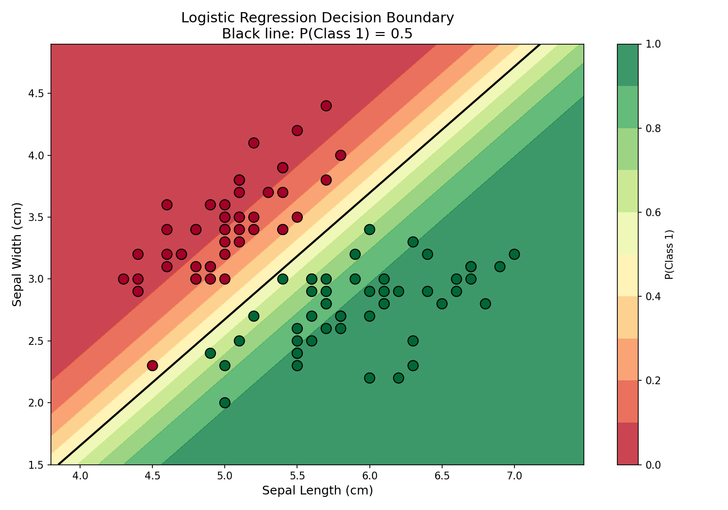
Decision Boundary Visualization

The true power of logistic regression becomes visible when plotting the decision boundary — the line where P(Class 1) = 0.5. This visualization shows how the model separates two classes in 2D feature space:

 1
 2
 3
 4
 5
 6
 7
 8
 9
10
11
12
13
14
15
16
17
18
19
20
21
22
23
24
25
26
27
28
29
30
31
32
33
34
35
36
37
38
39
40
41
42
43
44
45
46
47

import numpy as np
import matplotlib.pyplot as plt
from sklearn.linear_model import LogisticRegression
from sklearn.datasets import load_iris

# Load data (use only 2 features for visualization)
iris = load_iris()
X = iris.data[:100, :2]  # Sepal length & width, first 2 classes
y = iris.target[:100]

# Train model
clf = LogisticRegression()
clf.fit(X, y)

# Create mesh grid for decision boundary
h = 0.02
x_min, x_max = X[:, 0].min() - 0.5, X[:, 0].max() + 0.5
y_min, y_max = X[:, 1].min() - 0.5, X[:, 1].max() + 0.5
xx, yy = np.meshgrid(np.arange(x_min, x_max, h),
                     np.arange(y_min, y_max, h))

# Predict probabilities for each point in the mesh
Z = clf.predict_proba(np.c_[xx.ravel(), yy.ravel()])[:, 1]
Z = Z.reshape(xx.shape)

# Plot
fig, ax = plt.subplots(figsize=(10, 7))

# Probability contours
contour = ax.contourf(xx, yy, Z, levels=np.linspace(0, 1, 11), 
                       cmap='RdYlGn', alpha=0.8)
plt.colorbar(contour, label='P(Class 1)')

# Decision boundary (P = 0.5)
ax.contour(xx, yy, Z, levels=[0.5], colors='black', linewidths=2)

# Data points
scatter = ax.scatter(X[:, 0], X[:, 1], c=y, cmap='RdYlGn', 
                     edgecolors='black', s=100)

ax.set_xlabel('Sepal Length (cm)', fontsize=12)
ax.set_ylabel('Sepal Width (cm)', fontsize=12)
ax.set_title('Logistic Regression Decision Boundary\n'
             'Black line: P(Class 1) = 0.5', fontsize=14)
plt.tight_layout()
plt.savefig('assets/decision_boundary.png', dpi=150)
plt.show()

Deep Dive

This section addresses common questions and practical considerations when applying logistic regression.

Q1: Logistic regression vs. Perceptron?

Key insight: Logistic regression is preferred when probability estimates are needed, or when a smooth optimization landscape is desired.

Q2: What if classes are imbalanced?

Imbalanced datasets (e.g., 95% class 0, 5% class 1) can bias the model toward the majority class.

Solutions:

• Use class_weight='balanced' in sklearn — automatically adjusts weights inversely proportional to class frequencies
• Adjust the decision threshold — instead of 0.5, use a threshold that optimizes F1-score or precision/recall
• Resample the data — oversample minority class (SMOTE) or undersample majority class
• Use appropriate metrics — precision, recall, F1-score, or AUC-ROC instead of accuracy

1
2

# Example: handling imbalanced classes
clf = LogisticRegression(class_weight='balanced')

Q3: Why cross-entropy and not squared error?

Cross-entropy has nicer gradients for probability outputs.

Squared error can have very flat gradients near 0 and 1, making learning slow and potentially causing the model to get stuck.

Q4: Do features need to be scaled?

Yes, feature scaling is recommended for logistic regression, especially when using gradient descent.

1
2
3
4
5

from sklearn.preprocessing import StandardScaler

scaler = StandardScaler()
X_train_scaled = scaler.fit_transform(X_train)
X_test_scaled = scaler.transform(X_test)

Q5: How to prevent overfitting?

Logistic regression can overfit, especially with many features or when features are correlated.

Regularization:

• L2 (Ridge): $L + \lambda \sum w_j^2$ — shrinks all weights toward zero
• L1 (Lasso): $L + \lambda \sum |w_j|$ — encourages sparsity (some weights become exactly zero)

1
2
3
4
5

# L2 regularization (default)
clf = LogisticRegression(C=0.1)  # smaller C = stronger regularization

# L1 regularization (requires compatible solver)
clf = LogisticRegression(penalty='l1', solver='saga', C=0.1)

Q6: Logistic regression vs. other classifiers?

Summary

Key Formulas

Key Takeaways

1. Sigmoid transforms linear output to probability — essential for classification tasks
2. Cross-entropy loss provides better gradients than MSE for probability outputs
3. Decision boundary is a hyperplane defined by $\boldsymbol{w}^T \boldsymbol{x} = 0$
4. Multi-class can be handled via OvR (K binary classifiers) or Softmax
5. Regularization (L1/L2) prevents overfitting and improves generalization

When to Use Logistic Regression

References

• Bishop, C. “Pattern Recognition and Machine Learning” - Chapter 4
• sklearn Logistic Regression
• Cox, D.R. (1958). “The Regression Analysis of Binary Sequences”