Welcome to the first installment of The Shape of Sound, a blog series dedicated to demystifying the invisible world of acoustics. Based on the seminal works Modern Acoustics Theory Basis by the renowned physicist Ma Dayou and Theoretical Acoustics and Engineering Applications by He Lin et al., this series will take you from the fundamental physics of waves to the cutting-edge engineering of silence.

Today, we start at the very beginning: What exactly is sound, where did our understanding of it come from, and how do we describe it mathematically?

A Brief History: From Tuning Pipes to Galileo

Acoustics is arguably one of the oldest branches of science, originally rooted in the human fascination with language and music. Long before we understood frequency or wavelengths, ancient civilizations were mastering the art of “tuning.”

• Ancient China: As early as the 11th century, Shen Kuo noted that the quality of a musical instrument depended on its “acoustics”—a term derived from listening. However, quantitative work began much earlier. In the 3rd century BC, the Lüshi Chunqiu recorded the standardization of pitch using the “Huang Zhong” (Yellow Bell) tube. By 1584, Zhu Zaiyu of the Ming Dynasty solved a problem that had plagued musicians for millennia by mathematically formulating the twelve-tone equal temperament, essentially creating the tuning system used in modern pianos today.
• The Scientific Revolution: Acoustics transitioned from art to science in the 17th century. Galileo Galilei (1564–1642) is often credited with opening the door to modern acoustics. In 1638, he analyzed the vibration of strings and pendulums, establishing the relationship between pitch and frequency (then called “vibration number”).
• The Age of Theory: By the 19th century, giants of physics like Rayleigh synthesized centuries of discovery. His monumental work, The Theory of Sound (1877), remains a classic, marking the maturity of classical acoustic theory.

Today, acoustics has expanded far beyond just “hearing.” It encompasses ultrasound, underwater acoustics, and noise control, yet the fundamental physics remains the same.

The Nature of Sound: It’s a Matter Wave

A common misconception is treating sound like light. However, they are fundamentally different. Light is an electromagnetic wave that can travel through a vacuum; sound is a matter wave.

Why Sound Needs a Medium

Sound requires a medium—gas, liquid, or solid. But why? The answer lies in how sound propagates.

Imagine a long chain of balls connected by springs. If you push the first ball, it compresses the spring next to it, which pushes the second ball, and so on. The disturbance travels down the chain—but no single ball moves very far.

This is exactly how sound works in air:

• The Balls represent the air molecules (providing Mass/Density, $\rho$).
• The Springs represent the air’s compressibility (providing Elasticity/Bulk Modulus, $K$).

This mechanical interplay—Mass (Inertia) vs. Spring (Restoring Force)—is the physical reality that we will translate into mathematics in the next section.

When an object vibrates (like a speaker cone or vocal cords), it pushes the adjacent air molecules. They compress, push the next layer of molecules, and so on. This chain reaction propagates outward as a wave.

Longitudinal Waves: Compression and Rarefaction

In fluids (air and water), sound waves are longitudinal. This means the particles vibrate in the same direction that the wave travels, creating alternating regions of:

• Compression: High density, molecules packed together
• Rarefaction: Low density, molecules spread apart

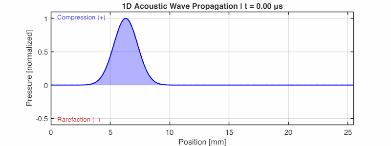
The animation below (generated using k-Wave) shows this beautifully: a pressure pulse propagating outward, with the blue shading indicating regions of compression.

The Mathematics of Commotion: Deriving the Wave Equation

How do physicists describe this invisible motion? The propagation of sound is governed by three fundamental laws of physics. By combining the mathematical expressions of these laws, we arrive at the “Holy Grail” of acoustics: the Wave Equation.

Here is the recipe for sound:

flowchart LR
    %% Define Styles
    classDef law fill:#A569BD,stroke:#8E44AD,color:white,rx:5,ry:5,stroke-width:2px;
    classDef process fill:#95A5A6,stroke:#7F8C8D,color:white,rx:5,ry:5;
    classDef result fill:#E74C3C,stroke:#C0392B,color:white,rx:5,ry:5,stroke-width:2px;
    
    subgraph Laws [Fundamental Laws]
        direction TB
        A("Conservation of Mass
(Continuity)"):::law
        B("Newton's 2nd Law
(Momentum)"):::law
        C("Thermodynamics
(Equation of State)"):::law
    end
    
    D("Eliminate ρ, v"):::process
    E("Wave Equation
$$ \nabla^2 p - \frac{1}{c_0^2}\frac{\partial^2 p}{\partial t^2} = 0 $$"):::result
    
    A --> D
    B --> D
    C --> D
    D --> E
    
    %% Style the subgraph
    style Laws fill:#FEF9E7,stroke:#F1C40F,stroke-width:2px,color:#7F8C8D

The Equation of Continuity (Conservation of Mass)

Imagine a tiny, fixed volume of air. Matter cannot be created or destroyed. Therefore, the net flow of mass into this tiny volume must equal the rate at which the density inside increases. $$ \frac{\partial \rho}{\partial t} + \nabla \cdot (\rho \boldsymbol{v}) = 0 $$

Translation: The change in density ($\rho$) over time is linked to the divergence of particle velocity ($\boldsymbol{v}$).

The Equation of Motion (Newton’s Second Law)

Force equals mass times acceleration ($F=ma$). In a fluid, the “force” comes from pressure differences. If the pressure on one side of our tiny volume is higher than the other, the air particles will accelerate toward the low-pressure side.

$$ \rho \frac{\partial \boldsymbol{v}}{\partial t} + \nabla p = 0 \quad \text{(Linearized version)} $$

Translation: The pressure gradient ($\nabla p$) drives the acceleration of the particles.

The Equation of State (Thermodynamics)

We need a rule to connect pressure ($p$) and density ($\rho$). In acoustics, sound propagation is usually an adiabatic process. This means the compression and expansion of air happen so fast that there is no time for heat to transfer between adjacent particles. $$ p = c_0^2 \rho’ $$

Translation: Pressure changes are directly proportional to density changes, scaled by the square of the speed of sound ($c_0$).

The Result: The Wave Equation

By mathematically combining these three equations (eliminating velocity and density variables), we are left with a single, elegant equation that describes how sound pressure varies in time and space:

$$ \nabla^2 p - \frac{1}{c_0^2} \frac{\partial^2 p}{\partial t^2} = 0 $$

This is the Wave Equation. It tells us that the spatial curvature of sound pressure ($\nabla^2 p$) is directly tied to its temporal acceleration, linked by the speed of sound. This equation is the foundation for nearly every problem in acoustics—from designing a concert hall to silencing a submarine.

What Can the Wave Equation Predict?

This single equation unlocks an enormous range of applications. Once you know how to solve it (using boundary conditions and source terms), you can:

• Simulate Room Acoustics: Predict how sound bounces inside a concert hall or recording studio.
• Design Mufflers: Calculate how an expansion chamber reflects exhaust noise back toward the engine.
• Model Ultrasound: Simulate focused ultrasound for medical imaging or therapy.
• Understand Holography: Reconstruct the sound field from microphone array data.

In the rest of this series, we will apply this equation to increasingly complex real-world problems.

What’s Next?

Now that we understand that sound is a physical pressure wave governed by Newton’s laws, how do we measure it? Why do we use that confusing “decibel” unit?

In the next post, “The Mystery of Decibels and Human Hearing,” we will bridge the gap between this raw physics and human perception, exploring why 0 dB isn’t “silence” and why distinct sounds don’t add up the way you think they should.

References:

• Ma Dayou, Modern Acoustics Theory Basis, Science Press, 2004.
• He Lin et al., Theoretical Acoustics and Engineering Applications, Science Press, 2006.