This blog explores the Lorenz attractor, a fascinating example of chaos theory, through numerical simulations. It delves into the mathematical foundations, explains key parameters, and demonstrates visualization techniques using various programming tools like Julia, Python, MATLAB, and COMSOL. The post compares methods like Euler and Dormand-Prince, highlighting their strengths and weaknesses, while showcasing the beauty and complexity of chaotic systems.
Introduction
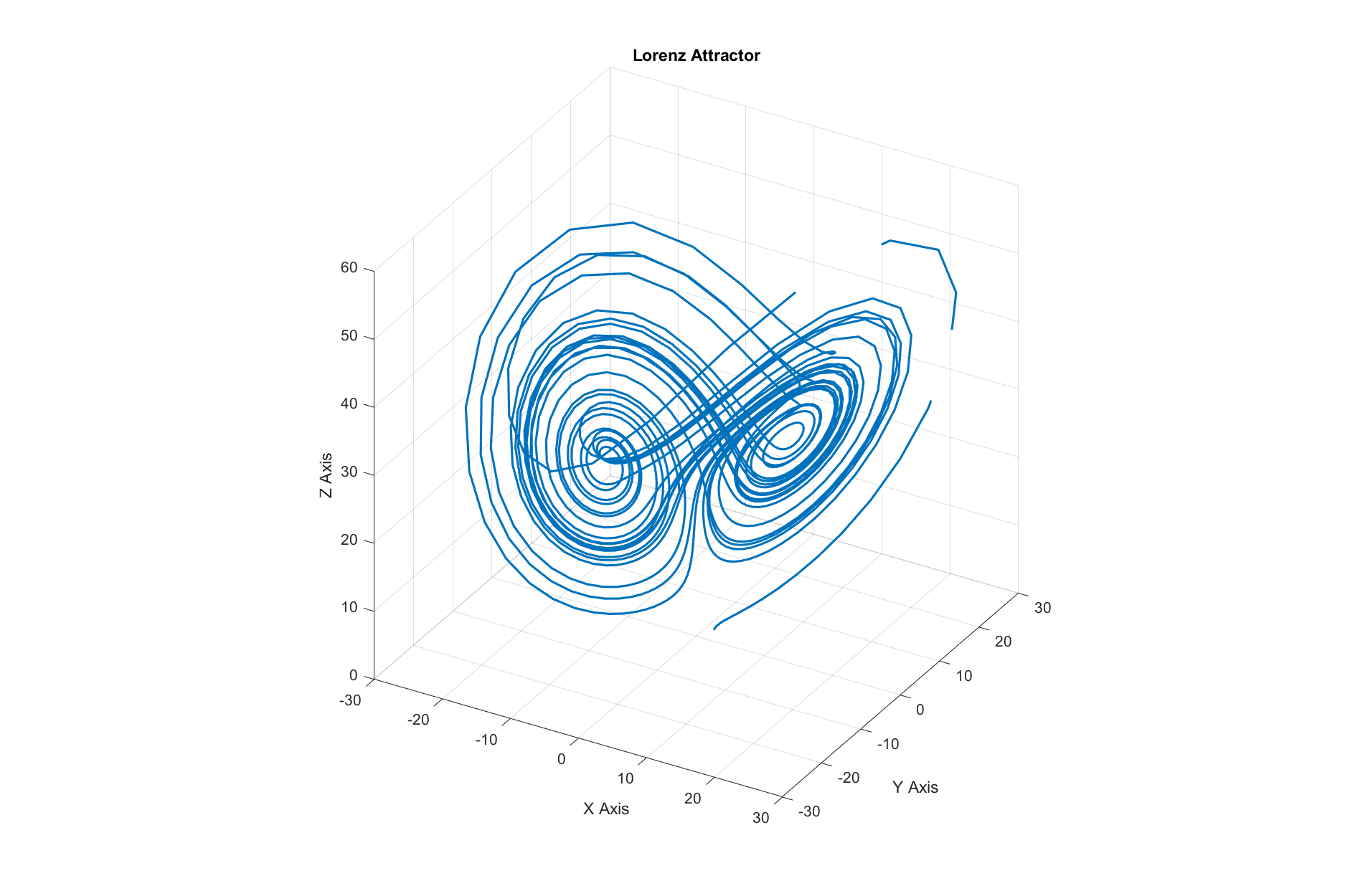
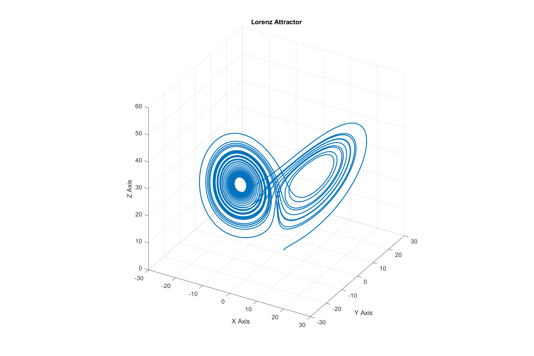
Lorenz attractor is a 3D structure that visualizes chaotic behavior, originally discovered by Edward Lorenz in 1963 while he was studying atmospheric convection (weather patterns). It is famous for being a “strange attractor.” This means that while the system is deterministic (it follows strict rules), its long-term behavior is unpredictable and never repeats itself. The trajectory loops around two points, creating a shape that famously resembles a butterfly.
From a technical standpoint, the Lorenz system is nonlinear, aperiodic, three-dimensional, and deterministic. While originally for weather, the equations have since been found to model behavior in a wide variety of systems, including lasers, dynamos, electric circuits, and even some chemical reactions
Here is the famous system:
$$
\begin{aligned}
\frac{dx}{dt} &= \sigma (y - x), \\
\frac{dy}{dt} &= x (\rho - z) - y, \\
\frac{dz}{dt} &= xy - \beta z.
\end{aligned}
$$
These equations describe how the state of the atmosphere changes over time ($t$).
$x$: The rate of convection (how fast the fluid is moving, proportional to the intensity of the convection).
$y$: The horizontal temperature difference (proportional to the temperature difference between the rising and falling air currents).
$z$: The vertical temperature gradient (proportional to the distortion of the vertical temperature profile).
The constants $\sigma, \rho, \beta$ are parameters representing physical properties of the system.
$\sigma$ is the
Prandtl number
. This is essentially the ratio of the fluid’s viscosity to its thermal conductivity. A high number means the fluid is thick and holds onto momentum (like oil), while a low number means heat spreads through it faster than it can physically move (like mercury).
$\rho$ is the
Rayleigh number
. It represents the temperature difference between the hot bottom and the cold top.
$\beta$ relates to the physical dimensions of the fluid layer itself. It describes the aspect ratio (width vs. height) of the circular currents in the fluid.
Visualization
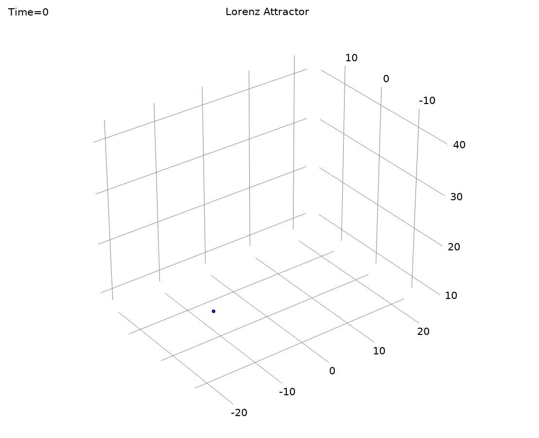
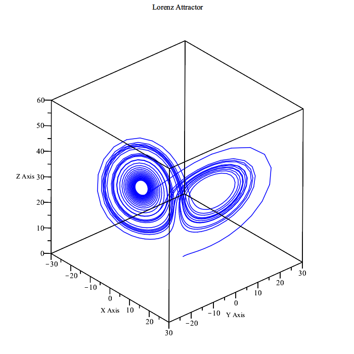
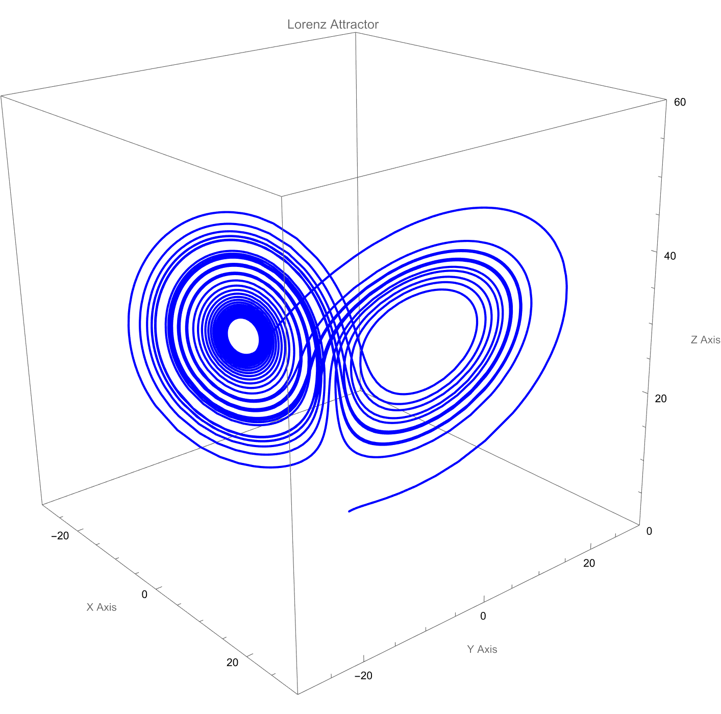
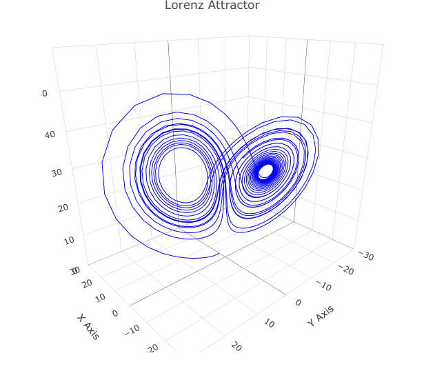
When $\rho=28$, $\sigma=10$, and $\beta=\dfrac{8}{3}$, the Lorenz system has chaotic solutions (but not all solutions are chaotic). Almost all initial points will tend to an invariant set — the Lorenz attractor — which is a strange attractor, a fractal, and a self-excited attractor with respect to all three equilibria. To simulate the Lorenz attractor, we use numerical methods to solve the equations. Two common methods are:
Euler Method: A simple and fast method, but less accurate for chaotic systems.
Dormand-Prince Method: A more advanced method (used in ode45 and RK45) that adapts the step size for better accuracy.
Below, we demonstrate how to visualize the Lorenz attractor using these methods in different programming languages and simulation tools.
% Lorenz Attractor using COMSOL with Dormand-Prince Methodimportcom.comsol.model.*importcom.comsol.model.util.*model=ModelUtil.create('Model');% ==================== 1. Global Parameters ====================params=model.param;params.set('sigma','10');params.set('rho','28');params.set('beta','8/3');params.set('dt','0.02');params.set('Tfinal','30');% ==================== 2. Component and Physics ====================model.component.create('comp1',true);comp=model.component('comp1');comp.geom.create('geom1',3);comp.physics.create('ge','GlobalEquations','geom1');ge=comp.physics('ge').feature('ge1');ge.set('name',{'u';'v';'w'});ge.set('equation',{'ut-sigma*(v-u)';'vt-rho*u+v+u*w';'wt-u*v+beta*w'});ge.set('initialValueU',[2;10;10]);% ==================== 3. Study and Solver ====================model.study.create('std1');study=model.study('std1');study.create('time','Transient');study.feature('time').set('tlist','range(0,dt,Tfinal)');model.sol.create('sol1');sol=model.sol('sol1');sol.attach('std1');sol.create('st1','StudyStep');sol.create('v1','Variables');sol.create('t1','Time');timeSolver=sol.feature('t1');timeSolver.set('tlist','range(0,dt,Tfinal)');timeSolver.set('odesolvertype','explicit');timeSolver.set('rkmethod','dopri5');study.runNoGen;% ==================== 4. Post-processing ====================model.result.create('pg1','PlotGroup3D');pg=model.result('pg1');pg.set('looplevel',{'last'});pg.create('traj1','PointTrajectories');traj=pg.feature('traj1');traj.set('expr',{'u','v','w'});traj.set('linetype','tube');traj.set('tuberadiusscaleactive',true);traj.set('tuberadiusscale',0.1);traj.create('col1','Color');traj.feature('col1').set('expr','sqrt(ut^2+vt^2+wt^2)');% ==================== 5. Save Model ====================mphsave(model,fullfile(pwd,'Lorenz_attractor_DormandPrince.mph'));
usingPlots# Define the Lorenz attractor@kwdefmutable structLorenzdt::Float64=0.02σ::Float64=10ρ::Float64=28β::Float64=8/3x::Float64=2y::Float64=1z::Float64=1end# Update the state of the Lorenz attractorfunctionstep!(l::Lorenz)dx=l.σ*(l.y-l.x)dy=l.x*(l.ρ-l.z)-l.ydz=l.x*l.y-l.β*l.zl.x+=l.dt*dxl.y+=l.dt*dyl.z+=l.dt*dzend# Create an instance of the Lorenz attractorattractor=Lorenz()# Initialize a 3D plotplt=plot3d(1,xlim=(-30,30),ylim=(-30,30),zlim=(0,60),title="Lorenz Attractor",marker=2,legend=false,xlabel="X Axis",ylabel="Y Axis",zlabel="Z Axis",size=(1200,800),)# Build an animated GIFanim=@animatefor_=1:1500step!(attractor)push!(plt,attractor.x,attractor.y,attractor.z)endevery10gif(anim,joinpath(pwd(),"lorenz_attractor_euler_jl.gif"),fps=30)
usingPlotsusingDifferentialEquations# Define the Lorenz attractor@kwdefmutable structLorenzdt::Float64=0.02σ::Float64=10ρ::Float64=28β::Float64=8/3x::Float64=2y::Float64=1z::Float64=1end# Define the Lorenz system for DifferentialEquations.jlfunctionlorenz!(du,u,p,t)σ,ρ,β=pdu[1]=σ*(u[2]-u[1])# dx/dtdu[2]=u[1]*(ρ-u[3])-u[2]# dy/dtdu[3]=u[1]*u[2]-β*u[3]# dz/dtend# Create an instance of the Lorenz attractorattractor=Lorenz()# Define initial conditions and solve the Lorenz systemu0=[attractor.x,attractor.y,attractor.z]p=(attractor.σ,attractor.ρ,attractor.β)tspan=(0.0,1500*attractor.dt)prob=ODEProblem(lorenz!,u0,tspan,p)sol=solve(prob,DP5(),saveat=attractor.dt)# Initialize a 3D plotplt=plot3d(1,xlim=(-30,30),ylim=(-30,30),zlim=(0,60),title="Lorenz Attractor",marker=2,legend=false,xlabel="X Axis",ylabel="Y Axis",zlabel="Z Axis",size=(1200,800),)# Build an animated GIFanim=@animatefor_=1:1500step!(attractor)push!(plt,attractor.x,attractor.y,attractor.z)endevery10gif(anim,joinpath(pwd(),"lorenz_attractor_dormandprince_jl.gif"),fps=30)
importnumpyasnpimportmatplotlib.pyplotaspltfrommatplotlib.animationimportFuncAnimation# Define the Lorenz attractor with default parametersclassLorenz:def__init__(self,dt=0.02,sigma=10,rho=28,beta=8/3,x=2,y=1,z=1):self.dt=dtself.sigma=sigmaself.rho=rhoself.beta=betaself.x=xself.y=yself.z=z# Update the state of the Lorenz attractor using the Euler methoddefstep(self):dx=self.sigma*(self.y-self.x)dy=self.x*(self.rho-self.z)-self.ydz=self.x*self.y-self.beta*self.zself.x+=self.dt*dxself.y+=self.dt*dyself.z+=self.dt*dzreturnself.x,self.y,self.z# Create an instance of the Lorenz attractorattractor=Lorenz()# Initialize a 3D plotfig=plt.figure(figsize=(12,8),dpi=100)ax=fig.add_subplot(111,projection="3d")ax.set_xlim(-30,30)ax.set_ylim(-30,30)ax.set_zlim(0,60)ax.set_title("Lorenz Attractor")ax.set_xlabel("X Axis")ax.set_ylabel("Y Axis")ax.set_zlabel("Z Axis")# Initialize the plot with an empty series(line,)=ax.plot([],[],[],lw=0.8,color="#007acc",alpha=0.9)(points,)=ax.plot([],[],[],marker="o",markersize=3,markerfacecolor="#00d2ff",markeredgecolor="black",markeredgewidth=0.6,alpha=0.9,)# Data storage for the animationx_data,y_data,z_data=[],[],[]# Update the plot for each framedefupdate(frame):globalx_data,y_data,z_datax,y,z=attractor.step()x_data.append(x)y_data.append(y)z_data.append(z)line.set_data(x_data,y_data)line.set_3d_properties(z_data)points.set_data(x_data,y_data)points.set_3d_properties(z_data)returnline,points# Create an animated GIFani=FuncAnimation(fig,update,frames=1500,interval=10,blit=True)# Save the animation as a GIFani.save("lorenz_attractor_euler_py.gif",writer="pillow",fps=30)
importnumpyasnpimportmatplotlib.pyplotaspltfromscipy.integrateimportsolve_ivpfrommatplotlib.animationimportFuncAnimation# Define the Lorenz attractor with default parametersclassLorenz:def__init__(self,dt=0.02,sigma=10,rho=28,beta=8/3,x=2,y=1,z=1):self.dt=dtself.sigma=sigmaself.rho=rhoself.beta=betaself.x=xself.y=yself.z=z# Function to define the Lorenz system for solve_ivpdefequations(self,t,state):x,y,z=statedx=self.sigma*(y-x)dy=x*(self.rho-z)-ydz=x*y-self.beta*zreturn[dx,dy,dz]# Create an instance of the Lorenz attractorattractor=Lorenz()# Define initial conditions and time span for the solveru0=[attractor.x,attractor.y,attractor.z]t_span=(0,1500*attractor.dt)t_eval=np.arange(0,1500*attractor.dt,attractor.dt)# Solve the Lorenz system using Dormand-Prince methodsol=solve_ivp(attractor.equations,t_span,u0,t_eval=t_eval,method="RK45")# Extract solution pointsx_data,y_data,z_data=sol.y# Initialize a 3D plotfig=plt.figure(figsize=(12,8),dpi=100)ax=fig.add_subplot(111,projection="3d")ax.set_xlim(-30,30)ax.set_ylim(-30,30)ax.set_zlim(0,60)ax.set_title("Lorenz Attractor")ax.set_xlabel("X Axis")ax.set_ylabel("Y Axis")ax.set_zlabel("Z Axis")# Initialize the plot with an empty series(line,)=ax.plot([],[],[],lw=0.8,color="#007acc",alpha=0.9)(points,)=ax.plot([],[],[],marker="o",markersize=3,markerfacecolor="#00d2ff",markeredgecolor="black",markeredgewidth=0.6,alpha=0.9,)# Function to update the plot for each framedefupdate(frame):line.set_data(x_data[:frame],y_data[:frame])line.set_3d_properties(z_data[:frame])points.set_data(x_data[:frame],y_data[:frame])points.set_3d_properties(z_data[:frame])returnline,points# Create an animated GIFani=FuncAnimation(fig,update,frames=len(t_eval),interval=10,blit=True)ani.save("lorenz_attractor_dormandprince_py.gif",writer="pillow",fps=30)
% Lorenz Attractor using Euler Method% Define parameters for the Lorenz attractordt=0.02;sigma=10;rho=28;beta=8/3;% Initial conditionsx=2;y=1;z=1;% Number of steps for the simulationnum_steps=1500;% Initialize arrays to store the trajectoryx_vals=zeros(1,num_steps);y_vals=zeros(1,num_steps);z_vals=zeros(1,num_steps);% Store initial conditionsx_vals(1)=x;y_vals(1)=y;z_vals(1)=z;% Euler method to update the Lorenz attractorfori=2:num_stepsdx=sigma*(y-x);dy=x*(rho-z)-y;dz=x*y-beta*z;x=x+dt*dx;y=y+dt*dy;z=z+dt*dz;x_vals(i)=x;y_vals(i)=y;z_vals(i)=z;end% Plot the Lorenz attractorfigure;plot3(x_vals,y_vals,z_vals,'LineWidth',1.5);axisequal;view(30,30);gridon;xlim([-30,30]);ylim([-30,30]);zlim([0,60]);title('Lorenz Attractor');xlabel('X Axis');ylabel('Y Axis');zlabel('Z Axis');set(gcf,'Position',[100,100,1200,800]);saveas(gcf,fullfile(pwd,'lorenz_attractor_euler_matlab.png'));
(* Lorenz Attractor using Dormand-Prince method in Mathematica *)(* Define the Lorenz attractor parameters *)dt=0.02;σ=10;ρ=28;β=8/3;(* Initial conditions *)x0=2;y0=1;z0=1;(* Define the Lorenz system *)lorenzSystem={x'[t]==σ(y[t]-x[t]),(* dx/dt *)y'[t]==x[t](ρ-z[t])-y[t],(* dy/dt *)z'[t]==x[t]y[t]-βz[t](* dz/dt *)};(* Initial conditions *)initialConditions={x[0]==x0,y[0]==y0,z[0]==z0};(* Time span *)tspan=1500dt;(* Solve the Lorenz system using NDSolve with ExplicitRungeKutta (Dormand-Prince) *)sol=NDSolve[Join[lorenzSystem,initialConditions],{x,y,z},{t,0,tspan},Method->{"ExplicitRungeKutta","DifferenceOrder"->5},MaxSteps->Infinity];(* Create the 3D plot *)ParametricPlot3D[Evaluate[{x[t],y[t],z[t]}/.sol],{t,0,tspan},PlotRange->{{-30,30},{-30,30},{0,60}},PlotLabel->"Lorenz Attractor",AxesLabel->{"X Axis","Y Axis","Z Axis"},PlotStyle->Blue,ImageSize->{1200,800},BoxRatios->{1,1,1},PlotPoints->1500]
# Load required packageslibrary(deSolve)library(plotly)# Define the Lorenz attractor parametersdt<-0.02sigma<-10rho<-28beta<-8/3# Initial conditionsx0<-2y0<-1z0<-1# Define the Lorenz systemlorenz<-function(t,state,parameters){with(as.list(c(state,parameters)),{dx<-sigma*(y-x)# dx/dtdy<-x*(rho-z)-y# dy/dtdz<-x*y-beta*z# dz/dtlist(c(dx,dy,dz))})}# Set up parameters and initial stateparameters<-c(sigma=sigma,rho=rho,beta=beta)state<-c(x=x0,y=y0,z=z0)# Time spantimes<-seq(0,1500*dt,by=dt)# Solve using Dormand-Prince methodsol<-ode(y=state,times=times,func=lorenz,parms=parameters,method="ode45")# Convert to data framesol_df<-as.data.frame(sol)# Create interactive 3D plot using plotlyfig<-plot_ly(sol_df,x=~x,y=~y,z=~z,type="scatter3d",mode="lines",line=list(color="blue",width=2))%>%layout(title="Lorenz Attractor",scene=list(xaxis=list(title="X Axis",range=c(-30,30)),yaxis=list(title="Y Axis",range=c(-30,30)),zaxis=list(title="Z Axis",range=c(0,60))))# Display the plotfig
Comparison of Tools and Methods
Method
Advantages
Disadvantages
Euler
Simple and fast
Less accurate for chaotic systems
Dormand-Prince
Adaptive step size, more accurate
Slower, more complex implementation
COMSOL
Built-in solver, easy visualization
Requires proprietary software
Julia
High performance, concise syntax
Requires familiarity with Julia
Python
Widely used, rich libraries
Slower than compiled languages
MATLAB
Excellent for numerical computation
Expensive, less flexible for animation
R
Good for statistical analysis
Limited support for 3D visualization
The choice of method depends on the trade-off between speed, accuracy, and the tools available.
Conclusion
The Lorenz attractor is a beautiful example of chaos theory, demonstrating how simple equations can produce complex, unpredictable behavior. In this blog, we explored various ways to visualize the attractor using different numerical methods and programming tools.
Each method has its strengths and weaknesses, and the choice depends on your goals and resources. Whether you’re a beginner or an expert, experimenting with the Lorenz attractor is a great way to learn about dynamical systems and numerical simulation.